Reading Execution Plans 1: Estimated vs Actual Plans, Operators and Join Algorithms

Version note: The T-SQL (Transact-SQL, Microsoft's dialect of SQL (Structured Query Language)) examples in this post were run on SQL Server 2025 CU10 (17.0.5035.5, compatibility level 170), and the C# examples with .NET 10 and Entity Framework Core (EF Core) 10.0.14.

Guess First

The customer detail page loads the customer's 2026 orders together with their items using EF Core's Include:

int customerId = 42;
var since = new DateTime(2026, 1, 1);
var orders = await db.Orders
    .Where(o => o.CustomerId == customerId && o.CreatedAt >= since)
    .Include(o => o.Items)
    .OrderByDescending(o => o.CreatedAt)
    .ToListAsync();
Console.WriteLine($"{orders.Count} orders, {orders.Sum(o => o.Items.Count)} items");

104 orders, 244 items

I ran the SQL EF Core generated on the server with the same parameter types (@customerId int, @since datetime2(7)) and captured the actual plan. The plan has eight operators, and SSMS (SQL Server Management Studio) puts a "Cost %" on each. Which operator do you think is the most expensive: the one with the highest percentage, or another one? Guess before looking at the figure below.

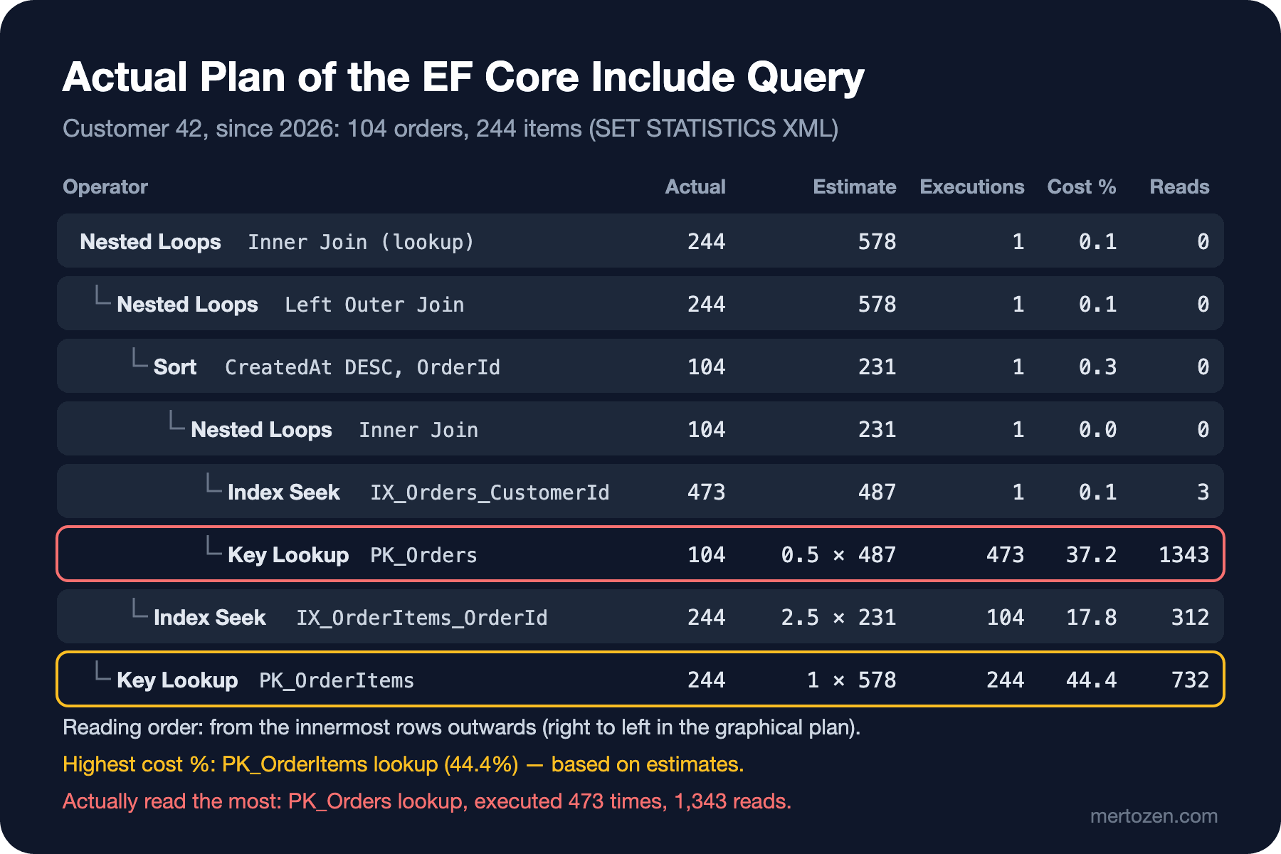
By cost percentage, the most expensive is the PK_OrderItems lookup (44.4%). The one that actually read the most pages, though, is the PK_Orders lookup: it executed 473 times and did 1,343 logical reads, more than half of all reads in the plan. That is because cost percentage is computed before execution, from estimates, and does not change even in the actual plan. In this post we will talk about how to get a plan, how to read it, the basic operators and the three join algorithms; and the most important habit will be this: first compare estimated and actual row counts.

How to Get a Plan

There are two kinds of plans. The estimated plan is compiled without running the query: operators, estimated row counts and costs. The actual plan is the same plan after execution: runtime information is added for every operator, such as the actual row count, how many times it ran (executions) and per-operator logical reads. The plan itself does not change; what changes is the measurements written on top of it.

/* estimated: the query does not run */
SET SHOWPLAN_XML ON;      /* or as text: SET SHOWPLAN_TEXT ON */

/* actual: the query runs and the plan comes back as a result */
SET STATISTICS XML ON;    /* or as text: SET STATISTICS PROFILE ON */
SET STATISTICS IO ON;     /* logical/physical reads per table */

/* the plan in the cache (estimated) */
SELECT qp.query_plan
FROM sys.dm_exec_query_stats AS qs
CROSS APPLY sys.dm_exec_query_plan(qs.plan_handle) AS qp;

/* the actual plan of the last execution (2019+, enabled per database) */
ALTER DATABASE SCOPED CONFIGURATION SET LAST_QUERY_PLAN_STATS = ON;
SELECT ps.query_plan
FROM sys.dm_exec_cached_plans AS cp
CROSS APPLY sys.dm_exec_query_plan_stats(cp.plan_handle) AS ps;

In graphical tools: in SSMS 22 (generally available on November 11, 2025), Ctrl+L opens the estimated plan and Ctrl+M the actual plan; Visual Studio Code's (VS Code) MSSQL (Microsoft SQL Server) extension can show plans graphically too. In this series I use the text form of the plan and values read from the XML (Extensible Markup Language) instead of screenshots, because they carry the same information and can be copied. The best source for a query's past plans in production is Query Store; we will open it up in post eight. If you want to learn the operators one by one with examples, Grant Fritchey's book SQL Server Execution Plans (3rd edition), published by Redgate as a free e-book, is a good reference.

Reading a Plan: Right to Left, Inside Out

The SQL EF Core generated is this:

SELECT [o].[OrderId], [o].[CreatedAt], [o].[Currency], [o].[CustomerId], [o].[OrderNumber], [o].[Status], [o].[TotalAmount],
       [o0].[OrderItemId], [o0].[BookId], [o0].[OrderId], [o0].[Quantity], [o0].[UnitPrice]
FROM [Orders] AS [o]
LEFT JOIN [OrderItems] AS [o0] ON [o].[OrderId] = [o0].[OrderId]
WHERE [o].[CustomerId] = @customerId AND [o].[CreatedAt] >= @since
ORDER BY [o].[CreatedAt] DESC, [o].[OrderId]

In the text form of the plan (SET STATISTICS PROFILE ON), the left columns are the actual row count, the execution count and the estimated row count:

    Rows Executes EstimateRows
     244        1    578.45044  |--Nested Loops(Inner Join, PASSTHRU:([IsBaseRow1001] IS NULL), OUTER REFERENCES:([o0].[OrderItemId]))
     244        1    578.45044       |--Nested Loops(Left Outer Join, OUTER REFERENCES:([o].[OrderId], [Expr1003]) WITH ORDERED PREFETCH)
     104        1    231.33427       |    |--Sort(ORDER BY:([o].[CreatedAt] DESC, [o].[OrderId] ASC))
     104        1    231.33427       |    |    |--Nested Loops(Inner Join, OUTER REFERENCES:([o].[OrderId], [Expr1002]) WITH UNORDERED PREFETCH)
     473        1    486.77777       |    |         |--Index Seek(OBJECT:([Orders].[IX_Orders_CustomerId] AS [o]), SEEK:([o].[CustomerId]=[@customerId]))
     104      473   0.47523591       |    |         |--Clustered Index Seek(OBJECT:([Orders].[PK_Orders] AS [o]), ... WHERE:([o].[CreatedAt]>=[@since]) LOOKUP)
     244      104    2.5004959       |    |--Index Seek(OBJECT:([OrderItems].[IX_OrderItems_OrderId] AS [o0]), SEEK:([o0].[OrderId]=[o].[OrderId]))
     244      244          1.0       |--Clustered Index Seek(OBJECT:([OrderItems].[PK_OrderItems] AS [o0]), ... LOOKUP)

In the graphical plan, data flows from right to left; in the text plan you read from the innermost lines outwards. This plan's story: IX_Orders_CustomerId found customer 42's 473 orders. Since CreatedAt is not in the index, a lookup into PK_Orders was done for each one (473 executions) and the date filter was applied there; 104 orders remained. These were sorted for the ORDER BY. Then for every order the items were searched in IX_OrderItems_OrderId (104 executions), and for BookId, Quantity and UnitPrice, which are not in the index, one more lookup was done per item (244 executions).

The thickness of arrows in the graphical plan shows the number of rows passing through: estimated rows in the estimated plan, actual rows in the actual plan. A thick arrow entering a thin operator, or conversely thousands of rows flowing through an arrow estimated at "1 row", is the first place to look. The Executes value matters at least as much as the row count: an operator with a small estimated cost that runs 473 times can be more expensive than an operator with a large cost that runs once.

Access Operators: Seek, Scan, Lookup

This is how you recognize in a plan the three access methods we saw in detail in post three. Index Seek / Clustered Index Seek: descends the B-tree to a specific key or range. Index Scan / Clustered Index Scan: reads the whole index (or part of it in a parallel plan); on a heap it is called Table Scan. Key lookup: "Key Lookup (Clustered)" in the graphical plan, a Clustered Index Seek carrying the word LOOKUP in the text plan; a trip per row to the clustered index for columns missing from the nonclustered index. Its heap equivalent is the RID (Row Identifier) Lookup.

In every access operator, look at two parts separately: SEEK: shows the range searched in the index, WHERE: the residual predicate applied afterwards to the rows read. In the PK_Orders lookup above, the date filter is in WHERE:: 473 rows were read and 369 thrown away. That is the clearest sign of a missing index.

Join Algorithms: Nested Loops, Merge Join and Hash Match

SQL Server can join two tables with three physical methods. I forced the same query (item quantities for the last 100,000 orders) with each one and measured; for a fair comparison, all of them ran single-threaded with MAXDOP 1:

SELECT o.OrderId, o.OrderNumber, SUM(oi.Quantity) AS Units
FROM dbo.Orders AS o
JOIN dbo.OrderItems AS oi ON oi.OrderId = o.OrderId
WHERE o.OrderId BETWEEN 900001 AND 1000000
GROUP BY o.OrderId, o.OrderNumber
OPTION (MAXDOP 1);              /* and OPTION (LOOP JOIN | MERGE JOIN | HASH JOIN, MAXDOP 1) */

Nested loops runs the inner input once for every row of the outer input. When the outer side is small and the inner side has an index, it is unbeatable; that is why every join in the Include plan is a nested loop. It needs no memory and starts returning the first row immediately. But as the outer side grows, its cost grows linearly: here 100,000 seeks, 306,259 logical reads. That is also why the "1 row" estimate in the previous post backfired so expensively.

Merge join needs both inputs sorted by the join key and walks them together like a zipper. If the inputs are already sorted thanks to an index, it is very cheap. If not, the optimizer adds a Sort, and a sort needs memory. In our plan the Orders side arrived in PK_Orders order, but the items came out of the aggregate in hash order and had to be sorted again.

Hash match builds a hash table in memory from the smaller input (build) and runs the larger input (probe) through it. It needs no order and is good for large, unsorted inputs. Its price is memory: if the build side turns out larger than estimated, the hash table spills to tempdb. Because it cannot produce output until the build is finished, it is blocking.

The Adaptive Join in the hint-free plan is the interesting one: the optimizer left the choice between nested loops and hash join to run time and picks one based on the actual row count on the build side. We will examine this operator, which runs in batch mode, in the next post together with memory grants and parallelism. Join hints are here only for measurement; forcing a join type in a production query means switching off the optimizer for every situation in which the data might change.

Aggregates: Stream Aggregate and Hash Aggregate

Grouping has two methods as well, and again the choice depends on whether the input is sorted:

SELECT CustomerId, COUNT(*) AS Orders FROM dbo.Orders WHERE CustomerId <= 1000 GROUP BY CustomerId OPTION (MAXDOP 1);
SELECT Status, COUNT(*) AS Orders FROM dbo.Orders GROUP BY Status OPTION (MAXDOP 1);

Table 'Orders'. Scan count 1, logical reads 650
    1000     1     1000.0  |--Stream Aggregate(GROUP BY:([Orders].[CustomerId]) DEFINE:([Expr1005]=Count(*)))
  371879     1  371868.03       |--Index Seek(OBJECT:([Orders].[IX_Orders_CustomerId]), SEEK:([Orders].[CustomerId] <= (1000)) ORDERED FORWARD)

Table 'Orders'. Scan count 1, logical reads 7601
       5     1        5.0  |--Hash Match(Aggregate, HASH:([Orders].[Status]) ...)
 1000000     1  1000000.0       |--Clustered Index Scan(OBJECT:([Orders].[PK_Orders]))

Because IX_Orders_CustomerId already delivers rows in CustomerId order, the stream aggregate totals each group in sequence: it needs no memory and emits the result as soon as a group ends. For Status there is no sorted input; the hash aggregate accumulates the five groups in an in-memory hash table. With few groups and a large input, hash aggregate is a good choice; with a very large number of groups, its memory needs and spill risk grow too.

The Main Signal: Estimated Versus Actual Rows

Back to the opening figure. Cost percentage is each operator's share of the total estimated I/O (Input/Output) and CPU (Central Processing Unit) cost. If the estimate is wrong, the percentage is wrong too; even in the actual plan this number is not recalculated. The PK_OrderItems lookup got 44.4% with an estimate of 578 executions, but actually ran 244 times and did 732 reads. The PK_Orders lookup got 37.2% with an estimate of 487, but actually ran 473 times and did 1,343 reads. The ranking flips.

So when reading a plan, look at these in order: big gaps between estimated and actual row counts (here 231 estimated and 104 actual for the date filter), operators that execute many times (Executes), residual predicates inside WHERE:, and per-operator logical reads. The diagnosis of this plan is clear: two lookups. Two indexes, one that moves the date filter into the index on orders and one that INCLUDEs the selected columns on items:

CREATE INDEX IX_Orders_Customer_Created ON dbo.Orders (CustomerId, CreatedAt);
DROP INDEX IX_OrderItems_OrderId ON dbo.OrderItems;
CREATE INDEX IX_OrderItems_OrderId ON dbo.OrderItems (OrderId) INCLUDE (BookId, Quantity, UnitPrice);

Table 'OrderItems'. Scan count 104, logical reads 359    /* before: 1089 */
Table 'Orders'. Scan count 1, logical reads 330          /* before: 1460 */

Because EF Core selects every column, the lookup on the Orders side did not disappear entirely, but it now happens only for the 104 orders that pass the filter; the lookup on items vanished completely. Total reads dropped from 2,549 to 689. The EF Core alternative is to project only the columns you really need with Select; the projection covered in the EF Core series' performance basics post directly makes index design easier here.

How SQL Server 2019/2022 differ: plan operators and how you read them are the same in all three versions. sys.dm_exec_query_plan_stats and LAST_QUERY_PLAN_STATS came with 2019. Seeing an Adaptive Join on rowstore tables requires batch mode on rowstore, which started in 2019 with compatibility level 150 and Enterprise edition. The PLAN PER VALUE suffixes you may see in plan text on 2022 and later belong to PSP (Parameter Sensitive Plan) optimization.

In Production

Getting an actual plan means running the query. Capturing the actual plan of a query containing UPDATE or DELETE in production "just to look" changes data. For these queries use the estimated plan, Query Store or sys.dm_exec_query_plan_stats, or do the work inside a transaction and roll back.

Do not rank by cost percentage. When comparing plans, use per-operator logical reads and Executes; in the actual plan these are real measurements.

Keep the plan. Comparing a query's "it was fast yesterday" plan with today's is the fastest way to a diagnosis; Query Store does this for you automatically.

Common Pitfalls

Mistaking the estimated plan for the actual one. The estimated plan has no "Actual Number of Rows"; the row counts you see there are estimates. To understand why a query is slow you need the actual plan, or at least STATISTICS IO.

Memorizing "scan bad, seek good". A seek that ran 100,000 times was far more expensive than a scan that ran once. Look at row counts, execution counts and reads more than at operator types.

"Fixing" the problem with join hints. A hint is a measurement tool. The permanent fix is usually the right index, the right statistics or rewriting the query.

Discussing a plan without looking at the SQL the ORM (Object-Relational Mapping) generated. Without seeing the SQL you cannot know that EF Core adds a LEFT JOIN and ORDER BY ..., [o].[OrderId] for Include, or that it sends the parameter as datetime2(7). Get the SQL with ToQueryString() or logging, and get the plan with that SQL.

A Small Experiment

★☆☆ Run the opening EF Core query for customer 2 (17,359 orders) and get the plan. Which operators changed? Are the lookups still there?

★★☆ Run the same query with AsSplitQuery(). How many SQL statements did EF Core send, and what does each plan look like? Compare the total logical reads with the single-query version.

★★★ Repeat the join comparison for WHERE o.OrderId BETWEEN 999901 AND 1000000 (100 orders). Which join was cheapest? What did the optimizer choose without hints, and why?

We left two topics in these plans for later: the memory that hash joins and sorts ask for (the memory grant), and the batch mode that Adaptive Join belongs to. In the next post we will read memory grant and spill warnings, parallel plans, exchange operators and the implicit conversion warning.