Train/Test Splits, Overfitting and Data Leakage: Why a Model Shines in Tests and Fails in Production

Version note: The code in this post was built and run with .NET 10, ML.NET 6.0 with the Microsoft.ML 6.0.0 package, and Microsoft.ML.FastTree 6.0.0. The data is synthetic Bookstore data produced by the series' seeded generator.

Guess First

You trained a delivery-time model for Bookstore, the online bookstore used as the shared example across this site's series, and it is off by 0.86 days on average on the test set. Someone on the team adds one more column and the error drops to 0.70 days, a 19 percent improvement. Would you ship this model right away? The added column is TrackingEventCount, the number of events in the carrier's tracking system.

If you read the previous post, you can guess the answer: this column only exists after the parcel is on its way, not at order time. The model looks better in testing because it sees part of the answer in the test set. In this post we use real measurements to see where this kind of fake success comes from and how to catch it.

Generalization and Baselines

What we expect from a model is not to memorize the orders it saw in training, but to predict well on new orders it has never seen. This is called generalization. The only way to measure it is to test the model on data you did not use in training. The simplest method is to split the data randomly in two: 80 percent train, 20 percent test.

This post is the first to use ML.NET, but we will open up the pipeline in the fourth post. For now, think of it as a box that takes a few columns and predicts delivery time with FastTree, a regression algorithm that trains decision trees one after another. The commands in this post read the data/orders_clean.csv file produced in the previous post; if you just cloned the repository, first run dotnet run --project tools/Bookstore.DataGen and then dotnet run --project src/Bookstore.ML.Lab -- clean. Let's add the packages and take the first measurement on split data:

/// <summary>Delivered orders only: cancelled orders have no label.</summary>
public static List<DeliveryInput> LoadDelivered()
{
    IDataView raw = Ml.Data.LoadFromTextFile<DeliveryInput>("data/orders_clean.csv", hasHeader: true, separatorChar: ',');
    return [.. Ml.Data.CreateEnumerable<DeliveryInput>(raw, reuseRowObject: false).Where(o => !o.IsCancelled)];
}
/// <summary>A small tree model; post 04 explains every step of this pipeline.</summary>
public static IEstimator<ITransformer> Pipeline(string[] numericFeatures, int leaves = 20, int trees = 100, int minLeaf = 10) =>
    Ml.Transforms.Conversion.ConvertType([new("Campaign", "IsCampaign"), new("Backorder", "HasBackorderItem")], DataKind.Single)
        .Append(Ml.Transforms.Categorical.OneHotEncoding([new("CarrierKey", "Carrier"), new("MethodKey", "ShippingMethod"),
            new("WarehouseKey", "Warehouse")]))
        .Append(Ml.Transforms.Concatenate("Features", ["CarrierKey", "MethodKey", "WarehouseKey", "Campaign", "Backorder",
            .. numericFeatures]))
        .Append(Ml.Regression.Trainers.FastTree(labelColumnName: "DeliveryDays", numberOfLeaves: leaves,
            numberOfTrees: trees, minimumExampleCountPerLeaf: minLeaf));

// 1) Random 80/20 split and two baselines
DataOperationsCatalog.TrainTestData random = Ml.Data.TrainTestSplit(all, testFraction: 0.2, seed: 7);
float trainMean = Ml.Data.CreateEnumerable<DeliveryInput>(random.TrainSet, false).Average(o => o.DeliveryDays);
List<DeliveryInput> randomTest = [.. Ml.Data.CreateEnumerable<DeliveryInput>(random.TestSet, false)];
Console.WriteLine($"rows: {rows.Count:N0}, train {random.TrainSet.GetRowCount() ?? Count(random.TrainSet):N0}, " +
                  $"test {randomTest.Count:N0}");
Console.WriteLine($"baseline 'always {trainMean:F2} days'  MAE {randomTest.Average(o => Math.Abs(o.DeliveryDays - trainMean)):F3}");
double ruleMae = randomTest.Average(o => Math.Abs(Rule(o) - o.DeliveryDays));
Console.WriteLine($"baseline rule from post 01      MAE {ruleMae:F3}");
ITransformer model = Pipeline(Basic).Fit(random.TrainSet);
Console.WriteLine($"tree model, random split       MAE {Mae(model, random.TestSet):F3}");

dotnet add src/Bookstore.ML.Lab package Microsoft.ML --version 6.0.0
dotnet add src/Bookstore.ML.Lab package Microsoft.ML.FastTree --version 6.0.0
dotnet run --project src/Bookstore.ML.Lab -- split

rows: 23,105, train 18,480, test 4,625
baseline 'always 2.58 days'  MAE 1.152
baseline rule from post 01      MAE 1.055
tree model, random split       MAE 0.860

The model's error of 0.860 days says nothing on its own. That is why we compare it with two baselines. The first is the laziest model, which tells every order the training set's mean (2.58 days): 1.152 days of error. The second is the hand-written rule from the first post: 1.055 days on the same test set. The model cuts the rule's error by about 18 percent. If a model cannot beat the mean baseline, either the features carry no information or there is a bug in the code; either way you need to know before looking at any other metric.

Train, Validation and Test

In a real project the data is split into three parts, not two. The train set is used to train the model. The validation set is used to compare and choose between models, feature sets and settings. The test set is opened only once, after all decisions are made, to measure the number you will report.

The reason for this split is that the moment you make a decision by looking at a dataset, that dataset becomes part of training. If you try ten models on the test set and pick the best, the test score of the chosen model is the score of the selection process, not of the model, and it is optimistic. The test set stands in for the unknown data the model will face in production; the less you touch it, the more honest its number is.

Overfitting and Underfitting

As model complexity grows, the training error always goes down. The validation error first goes down and then starts to rise. To see this, we vary the number of leaves each FastTree tree can have (numberOfLeaves) from 2 to 128. To make the effect visible, we train on only 1,500 rows and measure on 5,000:

IDataView all = Ml.Data.ShuffleRows(Ml.Data.LoadFromEnumerable(rows), seed: 5);
IDataView train = Ml.Data.TakeRows(all, 1500);
IDataView validation = Ml.Data.TakeRows(Ml.Data.SkipRows(all, 1500), 5000);
string[] features = [.. Basic, "TotalWeightKg", "OrderTotal"];
List<string> lines = ["leaves,train_mae,validation_mae"];
foreach (int leaves in new[] { 2, 3, 4, 6, 8, 12, 16, 24, 32, 48, 64, 96, 128 })
{
    ITransformer m = Pipeline(features, leaves: leaves, trees: 10, minLeaf: 1).Fit(train);
    double tr = Mae(m, train), va = Mae(m, validation);
    lines.Add(string.Create(CultureInfo.InvariantCulture, $"{leaves},{tr:F4},{va:F4}"));
    Console.WriteLine($"leaves {leaves,3}: train MAE {tr:F3}  validation MAE {va:F3}");
}

dotnet run --project src/Bookstore.ML.Lab -- complexity

leaves   2: train MAE 0.926  validation MAE 0.901
leaves   3: train MAE 0.836  validation MAE 0.843
leaves   4: train MAE 0.810  validation MAE 0.822
leaves   6: train MAE 0.796  validation MAE 0.819
leaves   8: train MAE 0.788  validation MAE 0.834
leaves  12: train MAE 0.768  validation MAE 0.863
leaves  16: train MAE 0.756  validation MAE 0.881
leaves  24: train MAE 0.733  validation MAE 0.890
leaves  32: train MAE 0.708  validation MAE 0.904
leaves  48: train MAE 0.675  validation MAE 0.904
leaves  64: train MAE 0.641  validation MAE 0.913
leaves  96: train MAE 0.590  validation MAE 0.929
leaves 128: train MAE 0.550  validation MAE 0.946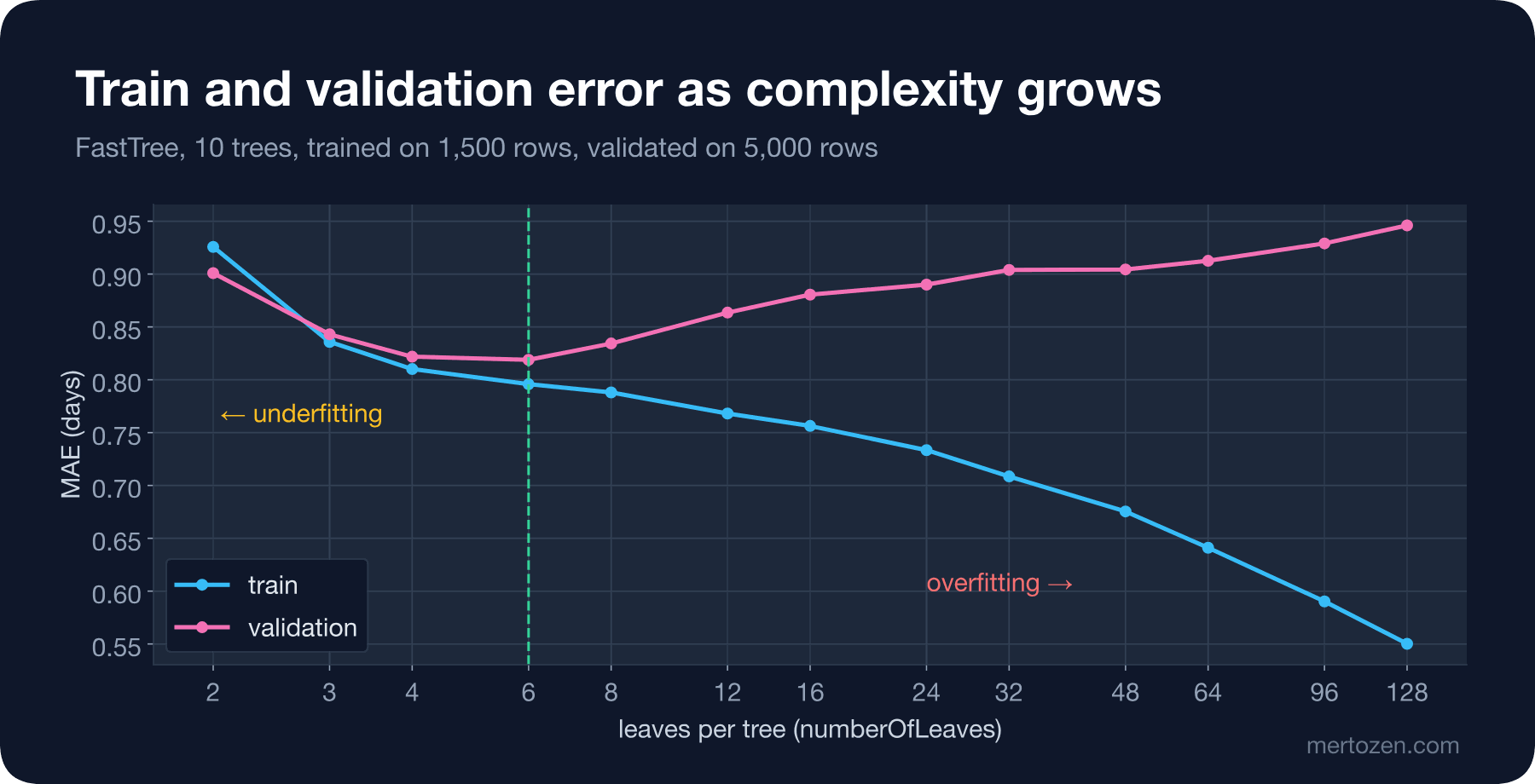

On the left of the chart, with 2-leaf trees, the model is too simple; both training and validation errors are high. This is underfitting: the model does not have the capacity to capture the relationship in the data. At 6 leaves the validation error reaches its lowest point (0.819). Moving right, the training error keeps falling down to 0.550, but the validation error climbs to 0.946. That is overfitting: the model has also learned the noise of 1,500 orders, and what it memorized does not help on new orders.

In the literature this balance is called the bias-variance trade-off. A simple model makes similar but systematically wrong predictions on every dataset (high bias). A complex model produces very different predictions when the training data changes a little (high variance). If you are curious about the mathematical side, An Introduction to Statistical Learning by James, Witten, Hastie and Tibshirani, published for free, is a good place to start. The practical lesson is simple: do not choose a model by its training error; watch the gap between training and validation error.

Target Leakage

Now back to the question from the opening. Adding TrackingEventCount to the feature list takes one line:

// 2) Target leakage: TrackingEventCount is only known after delivery
ITransformer leaky = Pipeline([.. Basic, "TrackingEventCount"]).Fit(random.TrainSet);
Console.WriteLine($"+ TrackingEventCount (leak)    MAE {Mae(leaky, random.TestSet):F3}");

+ TrackingEventCount (leak)    MAE 0.700

The error dropped from 0.860 to 0.700. Here the model is not learning delivery time but a by-product of the answer: the longer a parcel stays on the road, the more events pile up in the tracking system. This is called target leakage: the feature is fed by the label itself or by information created after the label is known. When this model goes to production, TrackingEventCount will be zero or empty at order time, and the 0.700 from testing will never be seen.

A classic example is return prediction. If you give a model that answers "will this order be returned?" the ReturnRequestedUtc column, or a feature derived from it such as "days until the return request", the model looks almost perfect, because that column is only filled in for returned orders. The best way to catch target leakage is not code but one question asked for every feature: in which system, and with what value, does this value exist at prediction time?

Time Leakage and Time-Based Splits

A random split picks test orders from anywhere in the two years. In production, however, the model will always predict future orders. To imitate that, we train on orders before 2026-05-01, test on the last six months and break the error down by month and carrier:

// 3) Time: train on the past, test on the last six months
DateTime cut = new(2026, 5, 1, 0, 0, 0, DateTimeKind.Utc);
IDataView past = Ml.Data.LoadFromEnumerable(rows.Where(o => o.OrderedAtUtc < cut));
List<DeliveryInput> future = [.. rows.Where(o => o.OrderedAtUtc >= cut)];
ITransformer timeModel = Pipeline(Basic).Fit(past);
Console.WriteLine($"tree model, time split         MAE {Mae(timeModel, Ml.Data.LoadFromEnumerable(future)):F3} " +
                  $"(train {Count(past):N0} before {cut:yyyy-MM-dd}, test {future.Count:N0})");
PredictionEngine<DeliveryInput, Prediction> engine = Ml.Model.CreatePredictionEngine<DeliveryInput, Prediction>(timeModel);
foreach (var g in future.GroupBy(o => (o.OrderedAtUtc.Month, o.Carrier == "CarrierB")).OrderBy(g => g.Key))
{
    double bias = g.Average(o => engine.Predict(o).Score - o.DeliveryDays);
    if (g.Key.Item2 || g.Key.Month is 5 or 10)
        Console.WriteLine($"  2026-{g.Key.Month:00} {(g.Key.Item2 ? "CarrierB" : "others  ")}  mean error {bias,6:F2} days ({g.Count()} orders)");
}

tree model, time split         MAE 0.864 (train 16,388 before 2026-05-01, test 6,717)
  2026-05 others    mean error  -0.05 days (646 orders)
  2026-05 CarrierB  mean error  -0.03 days (358 orders)
  2026-06 CarrierB  mean error  -0.74 days (350 orders)
  2026-07 CarrierB  mean error  -0.90 days (358 orders)
  2026-08 CarrierB  mean error  -0.82 days (359 orders)
  2026-09 CarrierB  mean error  -0.74 days (520 orders)
  2026-10 others    mean error  -0.13 days (698 orders)
  2026-10 CarrierB  mean error  -0.88 days (371 orders)

The total error (0.864) is almost the same as with the random split. But the details tell a different story: from June 2026 on, the model underestimates CarrierB orders by 0.7 to 0.9 days every month. On other orders the error is close to zero. We know that in the generator CarrierB became slower after that date; the model does not, because it never saw anything like it in the past data. Someone looking at a single total metric would never notice this. So always examine the error broken down into meaningful groups as well.

The first fix that comes to a developer's mind is giving the model the order date as a number (days since 2024-11-01, DaySerial). Measured with a random split, the result looks great:

// 3b) The order date as a feature: a random split lets the model peek at the future
List<DeliveryExtra> dated = [.. rows.Select(o => With(o, 0))];
var datedRandom = Ml.Data.TrainTestSplit(Ml.Data.LoadFromEnumerable(dated), testFraction: 0.2, seed: 7);
ITransformer dr = Pipeline([.. Basic, "DaySerial"]).Fit(datedRandom.TrainSet);
List<DeliveryExtra> drTest = [.. Ml.Data.CreateEnumerable<DeliveryExtra>(datedRandom.TestSet, false)];
ITransformer dt = Pipeline([.. Basic, "DaySerial"]).Fit(Ml.Data.LoadFromEnumerable(dated.Where(o => o.OrderedAtUtc < cut)));
List<DeliveryExtra> dtTest = [.. dated.Where(o => o.OrderedAtUtc >= cut)];
Console.WriteLine($"+ DaySerial, random split      MAE {Mae(dr, datedRandom.TestSet):F3}, CarrierB since June bias " +
                  $"{BiasB(dr, drTest):F2}");
Console.WriteLine($"+ DaySerial, time split        MAE {Mae(dt, Ml.Data.LoadFromEnumerable(dtTest)):F3}, CarrierB since June bias " +
                  $"{BiasB(dt, dtTest):F2}");
PredictionEngine<DeliveryInput, Prediction> randomEngine = Ml.Model.CreatePredictionEngine<DeliveryInput, Prediction>(model);
List<DeliveryInput> lateB = [.. randomTest.Where(o => o.Carrier == "CarrierB" && o.OrderedAtUtc >= new DateTime(2026, 6, 1))];
Console.WriteLine($"  random-split model on its own test rows, CarrierB since June: mean error " +
                  $"{lateB.Average(o => randomEngine.Predict(o).Score - o.DeliveryDays):F2} days ({lateB.Count} orders)");

+ DaySerial, random split      MAE 0.807, CarrierB since June bias -0.15
+ DaySerial, time split        MAE 0.913, CarrierB since June bias -1.09
  random-split model on its own test rows, CarrierB since June: mean error -0.63 days (410 orders)

With the random split the error drops to 0.807 and the post-June CarrierB error drops to -0.15; the problem looks solved. With the time-based split the same model is off by 0.913 and underestimates CarrierB by 1.09 days, worse than before the date was added. The difference comes from this: in the random split, 80 percent of the post-June orders sit in train, and the model learns the rule "if the date is after that day, CarrierB is slow" from the future. In production the future will never be in train. The last line also makes one thing clear: the random-split model without the date feature underestimates these orders by 0.63 days as well. So the random split does not hide the problem on its own; combined with the date feature, it does.

The rule is simple: if the data has time in it and the model will predict the future, do at least one evaluation with a time-based split. That split is what shows you that the world changed, a carrier's contract or a newly opened warehouse. We will get to how to monitor such changes in production in the tenth post.

Building Features by Looking at All the Data

The third kind of leakage is sneakier, because the feature looks completely legitimate. Adding each customer's past average delivery time as a feature makes sense: some customers live in a remote district and always receive late. The mistake is computing this average over all the data before the split:

// 4) A feature computed on all rows: the customer's average delivery time
List<DeliveryInput> train = [.. Ml.Data.CreateEnumerable<DeliveryInput>(random.TrainSet, false)];
Dictionary<string, float> avgAll = rows.GroupBy(o => o.CustomerId).ToDictionary(g => g.Key, g => g.Average(o => o.DeliveryDays));
Dictionary<string, float> avgTrain = train.GroupBy(o => o.CustomerId).ToDictionary(g => g.Key, g => g.Average(o => o.DeliveryDays));
foreach ((Dictionary<string, float> avg, string name) in new[] { (avgAll, "all rows (leak)"), (avgTrain, "train rows only") })
{
    IDataView tr = Ml.Data.LoadFromEnumerable(train.Select(o => With(o, avg.GetValueOrDefault(o.CustomerId, trainMean))));
    IDataView te = Ml.Data.LoadFromEnumerable(randomTest.Select(o => With(o, avg.GetValueOrDefault(o.CustomerId, trainMean))));
    ITransformer m = Pipeline([.. Basic, "CustomerAvgDays"]).Fit(tr);
    Console.WriteLine($"+ CustomerAvgDays from {name,-16} MAE {Mae(m, te):F3}");
}

+ CustomerAvgDays from all rows (leak)  MAE 0.837
+ CustomerAvgDays from train rows only  MAE 0.923

When the average is computed from all rows, the error drops to 0.837; without the feature it was 0.860. When it is computed from train rows only, the error rises to 0.923, so the feature makes the model worse. In the first case the test order's own delivery time is mixed into its customer's average. For customers with few orders, that average is almost the label itself. The second case is the honest measurement. In this dataset the customer average carries no real signal and only adds noise.

The same trap applies to every kind of preprocessing: the min and max of normalization, the mean used to fill missing values, the average label of a category. All of them must be learned from the training data only and merely applied to the test data. In ML.NET the way to guarantee that is to put these steps inside the pipeline; when you Fit the pipeline on the training set, these values are learned from there only. We will go into the details in the fifth post.

The Same Customer on Both Sides: samplingKeyColumnName

A random split treats rows as independent. But orders from the same customer are similar: same address, same district, same habits. If three orders of a customer are in train and one is in test, the model is predicting for a customer it partly knows. ML.NET's TrainTestSplit method takes a samplingKeyColumnName parameter for this; rows with the same value always land on the same side:

// 5) The same customer on both sides of the split
DataOperationsCatalog.TrainTestData grouped = Ml.Data.TrainTestSplit(all, testFraction: 0.2, samplingKeyColumnName: "CustomerId", seed: 7);
Console.WriteLine($"customers in both train and test: random {Overlap(random):N0}, " +
                  $"samplingKeyColumnName {Overlap(grouped):N0}");

customers in both train and test: random 2,035, samplingKeyColumnName 0

With the random split, 2,035 of the customers in the test set also have orders in train. With the split grouped by CustomerId that number is zero. Which one is right depends on the question you ask. If the model will always be used for existing customers, the random split is closer to reality. If you want it to be reliable for new customers too, or if you use customer-specific features, the grouped split gives a more honest number. In this series we will use the split grouped by customer.

Cross-Validation

A single split produces a number that depends on which rows land in the test set. k-fold cross-validation splits the data into k parts, uses one part as test and the rest as train each time, and produces k separate scores. In ML.NET this is a single call:

var folds = Ml.Regression.CrossValidate(all, Pipeline(Basic), numberOfFolds: 5, labelColumnName: "DeliveryDays",
    samplingKeyColumnName: "CustomerId", seed: 7);
double[] maes = [.. folds.Select(f => f.Metrics.MeanAbsoluteError)];
Console.WriteLine("5-fold MAE: " + string.Join("  ", maes.Select(m => m.ToString("F3", CultureInfo.InvariantCulture))));
Console.WriteLine($"mean {maes.Average():F3}, std {Std(maes):F3}");
// A small dataset: one split is a lottery
IDataView small = Ml.Data.TakeRows(Ml.Data.ShuffleRows(all, seed: 3), 400);
double[] single = [.. Enumerable.Range(1, 10).Select(seed =>
{
    var s = Ml.Data.TrainTestSplit(small, testFraction: 0.2, seed: seed);
    return Mae(Pipeline(Basic, minLeaf: 5).Fit(s.TrainSet), s.TestSet);
})];
Console.WriteLine($"400 rows, 10 different 80/20 splits: MAE min {single.Min():F3}, max {single.Max():F3}");
var smallCv = Ml.Regression.CrossValidate(small, Pipeline(Basic, minLeaf: 5), numberOfFolds: 5, labelColumnName: "DeliveryDays", seed: 7);
double[] cvMaes = [.. smallCv.Select(f => f.Metrics.MeanAbsoluteError)];
Console.WriteLine($"400 rows, 5-fold CV: mean {cvMaes.Average():F3}, std {Std(cvMaes):F3}");

dotnet run --project src/Bookstore.ML.Lab -- cv

5-fold MAE: 0.860  0.903  0.861  0.803  0.822
mean 0.850, std 0.039
400 rows, 10 different 80/20 splits: MAE min 1.005, max 1.629
400 rows, 5-fold CV: mean 1.222, std 0.174

On 23,105 rows the error of the five folds ranges from 0.803 to 0.903; the mean is 0.850 with a standard deviation of 0.039. With a single split you could have reported 0.803 or 0.903. On small data it gets much worse. On a 400-row subset, ten different random splits give results between 1.005 and 1.629: same model, same data, only luck differs. Cross-validation says 1.222 ± 0.174 here. That number is not certain either, but at least it honestly shows how large the uncertainty is.

Cross-validation has a cost: you train the model k times. On this dataset it takes a few seconds. On a large dataset with a slow algorithm it can take hours. Think about the scale the way the Big-O and Complexity series does: if the data doubles, training time at least doubles too, and k-fold multiplies that by k.

Common Pitfalls

The first pitfall is choosing a model by looking at the test set and then reporting the test score. Make the choice on a validation set or with cross-validation on the training data; open the test set once, at the very end.

The second is trusting a single split on small data. With a metric that moves between 1.0 and 1.6 on 400 rows, you cannot say "model A is better than model B". Look at the spread across folds.

The third is using a column that does not exist at prediction time as a feature. The column name can look innocent (TrackingEventCount, LastStatus, UpdatedAt); for every feature, ask "what would this value be at order time?"

The fourth is using only random splits on data with a time dimension. For a model that predicts the future, do at least one time-based evaluation and break the error down by time.

The fifth is doing preprocessing and feature building on all the data before the split. As the customer-average example showed, this can make a bad feature look good.

A Small Experiment

★☆☆ In the Splits.Complexity method, raise the number of trees from 10 to 100 and draw the curve again. Where does the number of leaves with the lowest validation error move?

★★☆ Build a time-based split by hand instead of CrossValidate: train on the first 12 months and test on month 13, then train on 13 months and test on month 14, and so on. Print the error for each month and look at what happens after June 2026.

★★★ Produce target leakage for return prediction yourself: train a simple binary classification model with the IsReturned label and a feature derived from ReturnRequestedUtc, then remove that feature and measure again. We have not covered classification metrics yet; for now look at how much accuracy changes, and in the seventh post we will discuss why these numbers are misleading.

In the next post we open up the pipeline we used as a box here: MLContext, the input class and [LoadColumn], the lazy nature of IDataView, the difference between an estimator and a transformer, the first SDCA model, PredictionEngine for a single prediction, and saving the model to a file and loading it back.