Regression and Its Metrics: Linear Regression, Gradient Boosting, MAE, RMSE and R²

Version note: The code in this post was built and run with .NET 10, ML.NET 6.0 with the Microsoft.ML 6.0.0 package, Microsoft.ML.FastTree 6.0.0 and Microsoft.ML.LightGbm 6.0.0. The data is synthetic Bookstore data produced by the series' seeded generator.

Guess First

We keep the feature pipeline we built in the previous post for Bookstore, the online bookstore used as the shared example across this site's series, fixed and attach four different trainers to its end: a linear model (SDCA) and three tree-based models (FastTree, FastForest, LightGBM). Tree-based gradient boosting models are known to usually give the best results on tabular data. Which one do you think wins on this data? How big will the difference be?

The second question is about metrics. 21 of the 4,489 orders in the test set, less than half a percent, are lost parcels that were found weeks later. If you remove these 21 rows from the test set, how much do MAE, RMSE and R² change?

Linear Regression and the Loss Function

Linear regression makes a prediction as a weighted sum of the features: each feature has a weight, plus a constant bias. Its simplest form with a single feature for delivery time is "days = w × distance + b". Training means finding the best values for w and b. What defines "best" is called the loss function. The most common loss in regression is the mean of the squared errors, MSE, the mean squared error.

Squaring has two consequences. Positive and negative errors do not cancel each other out. And large errors are punished disproportionately: a 10-day error produces not 10 but 100 times the loss of a 1-day error. This second property will come up later in this post when we talk about lost parcels.

Writing Gradient Descent by Hand

To see how the model finds w and b, let's put ML.NET aside and write our own loop. We predict delivery time from distance for Standard orders with no out-of-stock book. We divide the distance by 1,000 to keep the numbers small; remember the normalization lesson from the previous post:

(double X, double Y)[] points = [.. OrderRow.Load("data/orders_clean.csv")
    .Where(o => o.DeliveryDays is not null && o.ShippingMethod == "Standard" && !o.HasBackorderItem)
    .Select(o => (o.DistanceKm / 1000.0, o.DeliveryDays!.Value))];
foreach (double learningRate in new[] { 0.1, 0.5, 1.0 })
{
    double w = 0, b = 0;
    Console.WriteLine($"learning rate {learningRate}:");
    for (int epoch = 0; epoch <= 300; epoch++)
    {
        double gradW = 0, gradB = 0, loss = 0;
        foreach ((double x, double y) in points)
        {
            double error = w * x + b - y;      // prediction minus truth
            loss += error * error;
            gradW += 2 * error * x;
            gradB += 2 * error;
        }
        loss /= points.Length;
        if (epoch is 0 or 1 or 2 or 5 or 20 or 100 or 300)
        {
            Console.WriteLine($"  epoch {epoch,3}: MSE {loss,11:G6}   w {w,10:G5}   b {b,10:G5}");
        }
        w -= learningRate * gradW / points.Length;
        b -= learningRate * gradB / points.Length;
    }
}
// The exact least-squares answer for one feature, for comparison
double mx = points.Average(p => p.X), my = points.Average(p => p.Y);
double slope = points.Sum(p => (p.X - mx) * (p.Y - my)) / points.Sum(p => (p.X - mx) * (p.X - mx));
Console.WriteLine($"closed form: w {slope:F4}   b {my - slope * mx:F4}   ({points.Length:N0} orders)");

dotnet run --project src/Bookstore.ML.Lab -- gd

learning rate 0.1:
  epoch   0: MSE     10.3813   w          0   b          0
  epoch   1: MSE      7.7049   w    0.17197   b     0.5203
  epoch   2: MSE     6.06582   w    0.30848   b    0.92683
  epoch   5: MSE     4.06998   w    0.57402   b     1.6856
  epoch  20: MSE     3.46646   w    0.90516   b      2.337
  epoch 100: MSE     3.45271   w     1.2013   b     2.2647
  epoch 300: MSE     3.45191   w     1.2894   b     2.2374
learning rate 0.5:
  epoch   0: MSE     10.3813   w          0   b          0
  epoch   1: MSE     3.52897   w    0.85987   b     2.6015
  epoch   2: MSE     3.47234   w    0.83308   b     2.3586
  epoch   5: MSE     3.46336   w    0.94932   b     2.3428
  epoch  20: MSE     3.45261   w     1.2072   b     2.2628
  epoch 100: MSE     3.45191   w     1.2918   b     2.2366
  epoch 300: MSE     3.45191   w     1.2919   b     2.2366
learning rate 1:
  epoch   0: MSE     10.3813   w          0   b          0
  epoch   1: MSE      13.001   w     1.7197   b      5.203
  epoch   2: MSE     16.6254   w   -0.10718   b   -0.97154
  epoch   5: MSE     38.1176   w     2.7589   b     7.6923
  epoch  20: MSE     4396.67   w    -17.541   b    -58.466
  epoch 100: MSE 7.21825E+14   w -7.6295E+06   b -2.4607E+07
  epoch 300: MSE  7.8987E+42   w -7.981E+20   b -2.574E+21
closed form: w 1.2919   b 2.2366   (18,931 orders)

The logic of gradient descent is this: at each step, compute the slope (gradient) of the loss with respect to w and b and move both a little in the opposite direction of the slope. The learning rate decides how far to move. At 0.1 the model goes in the right direction but slowly: after 300 epochs w is still 1.2894, while the exact answer is 1.2919. At 0.5 it reaches the exact answer in 100 epochs. At 1.0 every step overshoots the valley and lands on the opposite slope; the loss grows at every step and after 300 epochs reaches the 7.8987E+42 shown in the output. The model diverged.

The result can be read too: every 1,000 km adds about 1.29 days to the delivery time, and even at zero distance there is a floor of 2.24 days. MSE staying at 3.45 shows that a single feature explains a small part of delivery time. SDCA does the same job, but with hundreds of features, smart step selection and regularization. Regularization limits overfitting by penalizing weights that grow too large.

Tree-Based Models

A decision tree splits the data with successive questions: "is the waiting time more than 40 hours?", "is there an out-of-stock book?", "is the distance more than 650 km?". In each leaf, the mean of the orders in that region becomes the prediction. A single tree overfits quickly, so in practice ensembles of trees are used. ML.NET offers three options:

• FastTree: in the words of the ML.NET documentation, an implementation of the MART gradient boosting algorithm. Trees are trained in sequence; each new tree tries to correct the error made by the sum of the previous trees.
• FastForest: the random forest approach. Trees are trained independently on different random subsets of the data and the features, and their predictions are averaged.
• LightGBM: Microsoft's open-source gradient boosting library; ML.NET wraps it in the Microsoft.ML.LightGbm package. It trains fast on large data by bucketing feature values into histogram bins.

The reasons trees are strong on tabular data are the ones we saw in the previous post: they find feature interactions on their own ("Friday and after 3 pm"), they are not affected by scale, and they capture non-linear relationships with thresholds.

Same Pipeline, Four Trainers

We train the four trainers with the full pipeline from the previous post on the same 80/20 split grouped by customer:

Dictionary<string, IEstimator<ITransformer>> trainers = new()
{
    ["SDCA"] = ml.Regression.Trainers.Sdca(new SdcaRegressionTrainer.Options
    {
        LabelColumnName = "DeliveryDays", FeatureColumnName = "Features", NumberOfThreads = 1,
    }),
    ["FastTree"] = ml.Regression.Trainers.FastTree(labelColumnName: "DeliveryDays", featureColumnName: "Features"),
    ["FastForest"] = ml.Regression.Trainers.FastForest(labelColumnName: "DeliveryDays", featureColumnName: "Features"),
    ["LightGBM"] = ml.Regression.Trainers.LightGbm(labelColumnName: "DeliveryDays", featureColumnName: "Features"),
};
Console.WriteLine($"{"trainer",-11}{"MAE",8}{"RMSE",8}{"R2",8}");
Dictionary<string, ITransformer> models = [];
foreach ((string name, IEstimator<ITransformer> trainer) in trainers)
{
    ITransformer model = FeatureLab.Full(trainer).Fit(train);
    RegressionMetrics m = ml.Regression.Evaluate(model.Transform(split.TestSet), labelColumnName: "DeliveryDays");
    Console.WriteLine($"{name,-11}{m.MeanAbsoluteError,8:F3}{m.RootMeanSquaredError,8:F3}{m.RSquared,8:F3}");
    models[name] = model;
}

dotnet add src/Bookstore.ML.Lab package Microsoft.ML.LightGbm --version 6.0.0
dotnet run --project src/Bookstore.ML.Lab -- compare

trainer         MAE    RMSE      R2
SDCA          0.525   1.691   0.342
FastTree      0.544   1.719   0.320
FastForest    0.611   1.722   0.317
LightGBM      0.536   1.703   0.332

The answer to the opening question: SDCA wins on this data. Its MAE is 0.525, LightGBM 0.536, FastTree 0.544, FastForest 0.611. But that does not mean "linear models beat trees". In the previous post, when we built the HoursUntilProcessing feature from the day and the hour, we handed the linear model, as a ready-made number, the interaction the tree finds on its own. Without that feature, SDCA's cross-validation error was 0.637 and FastTree's 0.541. Algorithm choice and feature engineering are not independent. With good features a simple model may be enough; with raw features trees are much more forgiving.

When the difference is small, the decision comes down to other criteria. SDCA's model is a few kilobytes, each of its weights is readable and it is very fast to compute. Tree models consist of hundreds of trees and their files are larger. On this data there is also a platform difference: LightGBM is a native library, and the LightGBM 4.6.0 package on NuGet contains compiled files only for win-x64, linux-x64 and osx-x64. It does not run on an ARM64 machine or container. On Linux it also needs the OpenMP library: in the Ubuntu-based .NET SDK container my first attempt failed with a DllNotFoundException because libgomp.so.1 was missing, and it worked after installing the libgomp1 package. That is why I ran this comparison in a Linux x64 container. The SDCA, FastTree and FastForest results were identical on another machine as well. If your deployment environment is ARM64, you can rule out LightGBM from the start.

MAE, RMSE and R²

The three metrics in the table answer different questions. MAE, the mean absolute error, is how many days the prediction is off from the actual value on average. Its unit is days, and it is the easiest to explain to the business: "our predictions are off by half a day on average". RMSE, the root of the mean of the squared errors, is also in days but punishes large errors more heavily, because it is computed from squared errors. An RMSE much larger than the MAE shows that some of the errors are very large; here it is 1.70 against 0.53.

R² shows how much of the variation in the label the model explains. A model that tells every order the mean gets R² = 0, a perfect model gets 1. A model worse than the mean can get a negative R². Because R² has no unit, it looks comparable across different problems, but that is an illusion, as we will see shortly.

Which one to choose depends on the business question. If you promise the customer a date, a 2-day error and a 10-day error do not cost the same. An order 10 days late means a call to customer service, a return and a lost customer. If large errors are expensive, watch RMSE. If you report a single number, choose MAE. And add a business metric like the one in the first post: for what share of orders does the prediction land within one day of reality? If being late is worse than arriving early, also look at the sign of the average error.

Residual Analysis

A residual is the difference between the prediction and the actual value. The average residual can be close to zero while being systematically positive or negative in a particular group. To catch this we split the test set into meaningful groups and look at each group's mean error:

(string Group, Func<Scored, bool> Filter)[] groups =
[
    ("all test orders", _ => true),
    ("Express", s => s.ShippingMethod == "Express"),
    ("back-ordered", s => s.HasBackorderItem),
    ("campaign week", s => s.IsCampaign),
    ("campaign + back-ordered", s => s.IsCampaign && s.HasBackorderItem),
    ("waits > 40 h (weekend)", s => s.HoursUntilProcessing > 40),
    ("delivered in > 15 days", s => s.DeliveryDays > 15),
];

mean error (days)             SDCA  LightGBM  orders
all test orders              -0.01     -0.01    4489
Express                      -0.14     -0.09     734
back-ordered                 -0.21     -0.28     107
campaign week                 0.10      0.10     513
campaign + back-ordered       0.09     -0.40      12
waits > 40 h (weekend)        0.07      0.07     590
delivered in > 15 days      -22.55    -22.54      21

On the whole test set the mean error is -0.01: overall the model is neither optimistic nor pessimistic. In the groups the picture is different. Both models predict Express orders a bit short (-0.14 and -0.09 days). For the 107 orders with an out-of-stock book both models fall short by 0.2–0.3 days; the uncertainty in supply time is large and the model predicts it with an average. In campaign weeks both models predict 0.10 days too long. When a campaign and a stock shortage come together, LightGBM is off by -0.40 days, but that is only 12 orders, and drawing conclusions from such a small group would be wrong.

The last row is the most striking: for the 21 deliveries that took more than 15 days, both models predict 22.5 days too short on average. No feature announces a lost parcel at order time. These rows are not the model's mistake; they are an event the model cannot see. Residual analysis is less about fixing the model and more about learning where it can be trusted and where it cannot.

How Outliers Affect the Metrics

We measure the same predictions of the same LightGBM model twice: once on the whole test set and once without the 21 rows longer than 15 days. We also measure Express and Standard orders separately:

IDataView normal = ml.Data.FilterRowsByColumn(test, "DeliveryDays", upperBound: 15);
RegressionMetrics all = ml.Regression.Evaluate(model.Transform(test), labelColumnName: "DeliveryDays");
RegressionMetrics clean = ml.Regression.Evaluate(model.Transform(normal), labelColumnName: "DeliveryDays");
long lost = test.GetColumn<float>("DeliveryDays").Count(d => d > 15);
Console.WriteLine();
Console.WriteLine($"LightGBM, all test rows       : MAE {all.MeanAbsoluteError:F3}  RMSE {all.RootMeanSquaredError:F3}  R2 {all.RSquared:F3}");
Console.WriteLine($"without {lost} rows over 15 days : MAE {clean.MeanAbsoluteError:F3}  RMSE {clean.RootMeanSquaredError:F3}  R2 {clean.RSquared:F3}");
foreach (string method in new[] { "Express", "Standard" })
{
    IDataView subset = ml.Data.FilterByCustomPredicate<DeliveryInput>(normal, o => o.ShippingMethod != method);
    RegressionMetrics m = ml.Regression.Evaluate(model.Transform(subset), labelColumnName: "DeliveryDays");
    Console.WriteLine($"  only {method,-8}: MAE {m.MeanAbsoluteError:F3}  RMSE {m.RootMeanSquaredError:F3}  R2 {m.RSquared:F3}");
}

LightGBM, all test rows       : MAE 0.536  RMSE 1.703  R2 0.332
without 21 rows over 15 days : MAE 0.432  RMSE 0.602  R2 0.800
  only Express : MAE 0.363  RMSE 0.518  R2 0.829
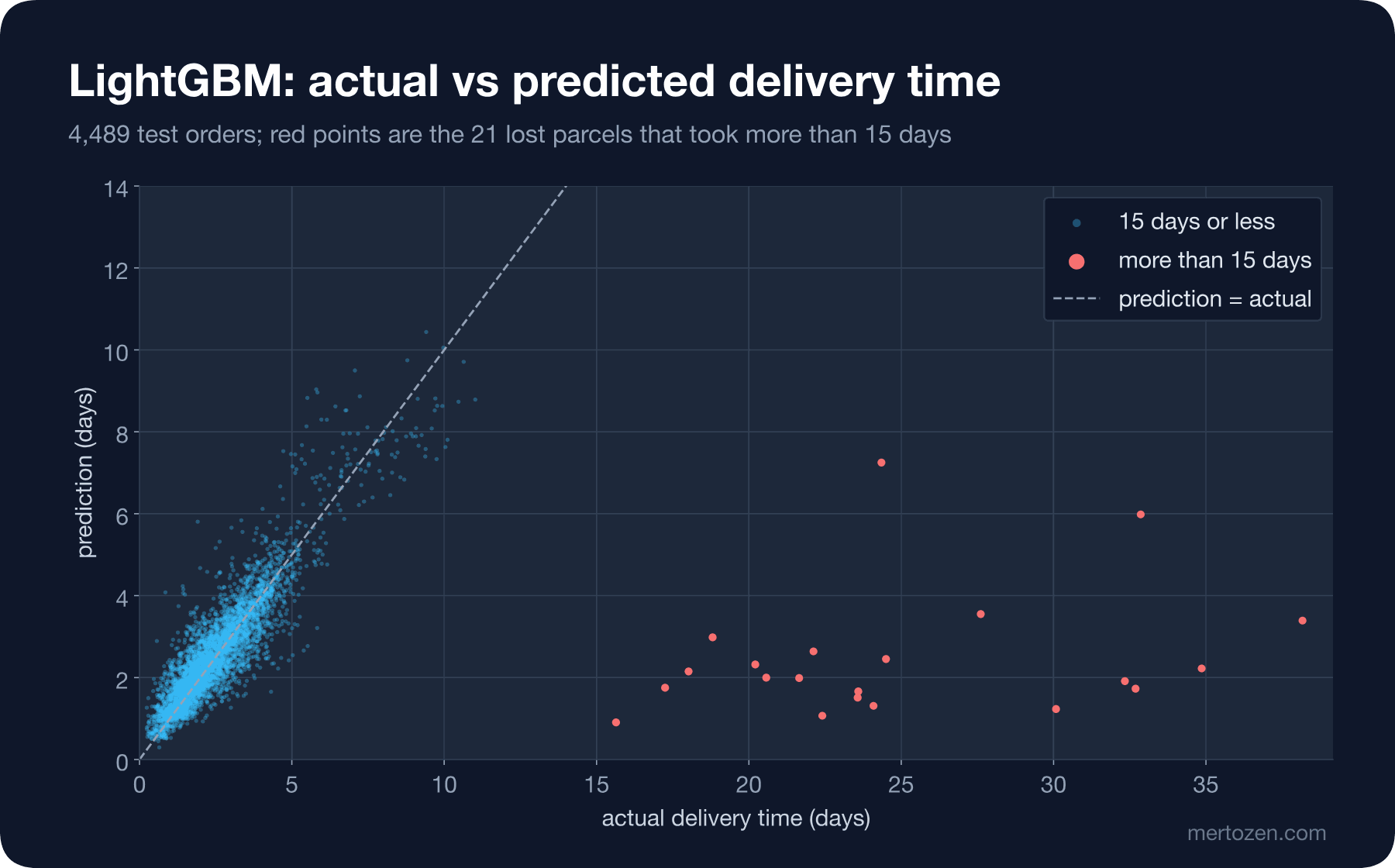
  only Standard: MAE 0.446  RMSE 0.617  R2 0.779

Here is the answer to the second question from the opening. Removing less than 0.5 percent of the test set lowers MAE from 0.536 to 0.432, cuts RMSE from 1.703 to 0.602, almost to a third, and raises R² from 0.332 to 0.800. The model did not change; what changed is which rows the metric looks at. The chart below shows why: predictions under 15 days cluster around the diagonal, while the 21 red points sit on the right, between predictions of 2–3 days and actual values of 15–38 days.

Two lessons follow. The first is about R²: the same model with the same predictions can score 0.33 or 0.80. R² is a property of the model and the test data together, not of the model alone. That is also why the R² of Express orders (0.829) being higher than Standard's (0.779) should be read with care. Do not interpret R² on its own; compare it together with MAE and RMSE on the same test set. The second is about outliers: quietly removing 21 rows from the test set and reporting 0.80 would not be honest. The right approach is to show both numbers and handle lost parcels with a separate process, for example an alert for parcels that do not move for a long time. Events like these are caught by a process, not by a model.

Extrapolation: Outside the Training Range

What does a model do outside the range it saw in training? Bookstore has a real example of this: individual orders have at most 12 books, while orders from the institutional order module have between 20 and 120. Let's train the model on individual orders only and ask about institutional ones:

IDataView individual = ml.Data.FilterRowsByColumn(data, "ItemCount", upperBound: 13);
List<DeliveryInput> institutional = [.. ml.Data.CreateEnumerable<DeliveryInput>(
    ml.Data.FilterRowsByColumn(data, "ItemCount", lowerBound: 20), false)];
ITransformer sdca = FeatureLab.Full(ml.Regression.Trainers.Sdca(new SdcaRegressionTrainer.Options
{
    LabelColumnName = "DeliveryDays", FeatureColumnName = "Features", NumberOfThreads = 1,
})).Fit(individual);
ITransformer gbm = FeatureLab.Full(ml.Regression.Trainers.LightGbm(labelColumnName: "DeliveryDays",
    featureColumnName: "Features")).Fit(individual);
var e1 = ml.Model.CreatePredictionEngine<DeliveryInput, DeliveryPrediction>(sdca);
var e2 = ml.Model.CreatePredictionEngine<DeliveryInput, DeliveryPrediction>(gbm);
Console.WriteLine();
Console.WriteLine($"trained on ItemCount <= 12; institutional orders in the data: {institutional.Count}, " +
                  $"mean {institutional.Average(o => o.DeliveryDays):F2} days");
double maeSdca = institutional.Average(o => Math.Abs(e1.Predict(o).PredictedDays - o.DeliveryDays));
double maeGbm = institutional.Average(o => Math.Abs(e2.Predict(o).PredictedDays - o.DeliveryDays));
Console.WriteLine($"  MAE on institutional orders: SDCA {maeSdca:F3}, LightGBM {maeGbm:F3}");

trained on ItemCount <= 12; institutional orders in the data: 310, mean 4.52 days
  MAE on institutional orders: SDCA 1.597, LightGBM 1.118

On institutional orders the error is 1.597 days for SDCA and 1.118 for LightGBM, two to three times the half day on the normal test set. The average delivery time of these orders is 4.52 days, because stock shortages are more frequent and offices do not receive deliveries at weekends. The model has never seen this world. The second experiment shows the difference more clearly. We train the model on orders closer than 1,000 km and ask about the same order at different distances:

// The same question for distance: train below 1,000 km, ask about Van (1,220 km from ANK-1)
IDataView near = ml.Data.FilterRowsByColumn(data, "DistanceKm", upperBound: 1000);
List<DeliveryInput> far = [.. ml.Data.CreateEnumerable<DeliveryInput>(
    ml.Data.FilterRowsByColumn(data, "DistanceKm", lowerBound: 1000), false)];
ITransformer sdcaNear = FeatureLab.Full(ml.Regression.Trainers.Sdca(new SdcaRegressionTrainer.Options
{
    LabelColumnName = "DeliveryDays", FeatureColumnName = "Features", NumberOfThreads = 1,
})).Fit(near);
ITransformer gbmNear = FeatureLab.Full(ml.Regression.Trainers.LightGbm(labelColumnName: "DeliveryDays",
    featureColumnName: "Features")).Fit(near);
var n1 = ml.Model.CreatePredictionEngine<DeliveryInput, DeliveryPrediction>(sdcaNear);
var n2 = ml.Model.CreatePredictionEngine<DeliveryInput, DeliveryPrediction>(gbmNear);
Console.WriteLine($"trained on DistanceKm < 1000; {far.Count} orders travel farther, mean {far.Average(o => o.DeliveryDays):F2} days");
DeliveryInput order = far.First(o => !o.HasBackorderItem && o.ShippingMethod == "Standard" && o.CustomerNote == "");
foreach (int km in new[] { 300, 600, 900, 1200, 1600 })
{
    order.DistanceKm = km;
    Console.WriteLine($"  {km,5} km: SDCA {n1.Predict(order).PredictedDays,5:F2}   LightGBM {n2.Predict(order).PredictedDays,5:F2}");
}
Console.WriteLine($"  MAE on the far orders: SDCA {far.Average(o => Math.Abs(n1.Predict(o).PredictedDays - o.DeliveryDays)):F3}, " +
                  $"LightGBM {far.Average(o => Math.Abs(n2.Predict(o).PredictedDays - o.DeliveryDays)):F3}");

trained on DistanceKm < 1000; 734 orders travel farther, mean 3.74 days
    300 km: SDCA  4.45   LightGBM  4.21
    600 km: SDCA  4.81   LightGBM  4.68
    900 km: SDCA  5.17   LightGBM  4.85
   1200 km: SDCA  5.53   LightGBM  4.85
   1600 km: SDCA  6.01   LightGBM  4.85
  MAE on the far orders: SDCA 0.701, LightGBM 0.795

Here the behavior of the two model families clearly diverges. SDCA continues the line: it adds about 0.36 days for every 300 km and says 6.01 days at 1,600 km. LightGBM flattens at 4.85 after 900 km; the leaves of the trees can do nothing but return the mean of the farthest region seen in training. Because the effect of distance really is linear in this data, SDCA is better on far orders (0.701 against 0.795). But if the relationship were not linear, the linear model "continuing the line" would be just as wrong. The practical conclusion: record the model's training range and flag requests that fall outside it in production. In the tenth post we will treat this as part of drift monitoring.

Common Pitfalls

The first pitfall is interpreting R² on its own. The same model can score 0.33 or 0.80 depending on the presence of a few outliers. Always report R² together with MAE and RMSE on the same test set.

The second is ignoring how outliers inflate RMSE or, the other way round, silently deleting them and reporting a nice number. Show both situations separately and discuss what the outlier means for the business.

The third is extrapolation. When a model that never saw an order with more than 12 books in training predicts a 120-book institutional order, the error triples. Know your training range and monitor requests that fall outside it.

The fourth is choosing the algorithm independently of the features. SDCA won in this post because we gave it the right feature in the previous one. Always compare algorithms on the same feature pipeline, and repeat the comparison when the features change.

The fifth is deciding by a single metric. A 0.011-day MAE difference may not be worth giving up model size, explainability or platform support.

A Small Experiment

★☆☆ Set the learning rate in the gradient descent loop to 0.9 and 0.95. At which value does the model start to diverge? Repeat the experiment without dividing the distance by 1,000 and see which learning rate works.

★★☆ Add a group by carrier to the Residuals method and measure CarrierB orders after June 2026 separately. Does the slowdown we saw in the third post show up in this model too? If it does, why?

★★★ Remove the lost parcels (deliveries longer than 15 days) from the training data and retrain the model, but do not touch the test set. How do MAE, RMSE and R² change? Write down the difference between removing outliers from training and removing them from evaluation.

In the next post we predict a class instead of a number: we build a binary classification model that predicts whether an order will be cancelled, and look at the confusion matrix, precision, recall, F1 and ROC-AUC, threshold selection and a multiclass model that predicts the topic from review text.