

When and How to Scale a Database? Measurement, Bottlenecks and the Scaling Ladder
You don't decide to scale a database before measuring p50/p95/p99 latency, throughput and what active sessions are waiting on; the first rung is usually query and index. Bookstore's order history query saturated at 187 requests/s with 64 clients, and one index took p99 from 653 ms to 5.6 ms. Finding the bottleneck with Little's Law, pg_stat_statements and DMVs, the scaling ladder, capacity estimation and SLOs.
Version note: The examples in this post were built and run on PostgreSQL 18.7 and SQL Server 2025 (CU10, 17.0.5035.5) with .NET 10, Npgsql 10.0.3 and Microsoft.Data.SqlClient 7.1.2. The measurements come from a single-machine lab; absolute timings will differ on your hardware, what matters is the ratios and the shape of the curve.
Guess First
Bookstore, the online bookstore used as the shared example across this site's series, plans for its order count to grow tenfold within a year. The product team's first question: "Will we need a bigger database server, replicas, or sharding?" The answer starts with a measurement. We have a PostgreSQL 18 database with 1 million orders and 2.5 million order lines. The query behind the "My orders" page fetches a customer's last 20 orders:
SELECT order_id, status, total_amount, created_at
FROM orders
WHERE customer_id = @customerId
ORDER BY created_at DESC
LIMIT 20;
We run this query with 1, 4, 16 and 64 concurrent clients for 20 seconds each. Guess: when the client count goes from 16 to 64, does the number of requests per second quadruple? What happens to the response time? Here is the measurement:
db=pg concurrency=1 requests=1152 errors=0
throughput=57.6 req/s p50=16.3 ms p95=22.9 ms p99=26.4 ms
db=pg concurrency=4 requests=2482 errors=0
throughput=124.0 req/s p50=31.9 ms p95=38.5 ms p99=43.6 ms
db=pg concurrency=16 requests=3113 errors=0
throughput=155.1 req/s p50=96.6 ms p95=170.8 ms p99=224.7 ms
db=pg concurrency=64 requests=3769 errors=0
throughput=186.9 req/s p50=327.5 ms p95=510.8 ms p99=653.4 ms
The client count grew 64 times, throughput only 3.2 times. Median response time jumped from 16 ms to 327 ms. Past a certain point the database doesn't do the work any faster; the work just waits in line. In this post we learn to read this curve, find the bottleneck and build the scaling ladder that answers "what's the next step?". Throughout the series we will climb the ladder one rung at a time with the same Bookstore scenario.
"The Database Is Slow" Is Not a Measurement
Turning a performance complaint into something useful takes three numbers. Throughput is the amount of work completed per unit of time (requests or transactions per second). Latency is how long a single request takes. A percentile tells you where in the latency distribution you're looking: p50 means half of the requests finished faster than this, p99 means one request in a hundred took longer. The average is no use here, because a few very slow requests disappear into it, yet those are exactly the requests users remember.
We take the measurement with a small .NET tool. The load command in Bookstore.ScaleLab starts the given number of workers; each one takes a connection from the pool, runs the query and records the elapsed time:
Task[] workers = Enumerable.Range(0, concurrency).Select(async worker =>
{
    Random random = new(worker);
    while (!stop.IsCancellationRequested)
    {
        long started = Stopwatch.GetTimestamp();
        try
        {
            await using DbConnection connection = Db.Create(db);
            await connection.OpenAsync();
            await using DbCommand command = connection.CreateCommand();
            command.CommandText = sql;
            DbParameter p = command.CreateParameter();
            p.ParameterName = "customerId";
            p.Value = random.Next(1, 100_001);
            command.Parameters.Add(p);
            await using DbDataReader reader = await command.ExecuteReaderAsync();
            while (await reader.ReadAsync()) { }
            // record the elapsed time for successful requests only
            latenciesMs.Add(Stopwatch.GetElapsedTime(started).TotalMilliseconds);
        }
        catch (DbException)
        {
            Interlocked.Increment(ref errors);
        }
    }
}).ToArray();

await Task.WhenAll(workers);
The percentile is a simple index calculation on the sorted array (the nearest-rank method):
static double Percentile(double[] sorted, int p) =>
    sorted.Length == 0 ? 0 : sorted[Math.Min(sorted.Length - 1, (int)Math.Ceiling(p / 100.0 * sorted.Length) - 1)];
To set up the lab and run the tool (PowerShell; generating the data takes a few minutes):
docker run -d --name bookstore-pg -p 5432:5432 -e POSTGRES_PASSWORD=<password> -e POSTGRES_DB=bookstore postgres:18 -c shared_preload_libraries=pg_stat_statements
Get-Content db/pg-schema.sql, db/pg-data.sql | docker exec -i bookstore-pg psql -q -U postgres -d bookstore
$env:BOOKSTORE_PG = "Host=localhost;Database=bookstore;Username=postgres;Password=<password>"
dotnet run --project src/Bookstore.ScaleLab -c Release -- load --db pg --concurrency 64 --seconds 20
This is not a load testing tool; its purpose is to see how a single query behaves under concurrency. Designing a real load test, its scenarios and tools are covered in the Performance and Load Testing series. What matters to us is the relationship behind the four lines above. By Little's Law, the average number of jobs in a system equals throughput multiplied by average time. At 64 clients, 186.9 requests/s times a median of about 0.33 s gives 61: almost all 64 clients are waiting for something at any moment. Once throughput hits its ceiling, every extra client only lengthens the queue and raises latency linearly. The point where the curve bends (between 4 and 16 clients in this lab) is the capacity limit for this query.
Finding the Bottleneck: Resource or Wait?
A database server chokes on one of five things: CPU, disk I/O, memory, locking/blocking or connection count. Instead of guessing which, we ask the server what its active sessions are doing right now. The tool has a sampler that runs every 200 ms while the load runs. For PostgreSQL the query is:
SELECT coalesce(wait_event_type || ':' || wait_event, 'CPU') AS wait, count(*)
FROM pg_stat_activity
WHERE state = 'active' AND backend_type = 'client backend' AND pid <> pg_backend_pid()
GROUP BY 1;
An active backend with an empty wait_event isn't waiting for anything; it's running on the CPU. The distribution for the 64-client run:
  active sessions on CPU: 46%
  active sessions on IO:AioIoCompletion: 29%
  active sessions on LWLock:BufferMapping: 23%
  active sessions on IPC:BgworkerShutdown: 0%
No lock waits, no connection errors. Time goes to CPU, to reading pages (AioIoCompletion, the asynchronous I/O introduced in 18) and to the internal lock used to look pages up in shared buffers (LWLock:BufferMapping). This table says "the server reads a lot of pages". pg_stat_statements tells us which query reads them:
SELECT left(query, 48) AS query, calls,
       round(mean_exec_time::numeric, 1) AS mean_ms,
       (shared_blks_hit + shared_blks_read) / calls AS blocks_per_call
FROM pg_stat_statements
WHERE dbid = (SELECT oid FROM pg_database WHERE datname = current_database())
ORDER BY total_exec_time DESC
LIMIT 2;
query | calls | mean_ms | blocks_per_call
--------------------------------------------------+-------+---------+-----------------
SELECT order_id, status, total_amount, created_a | 10516 | 156.4 | 16665
DISCARD ALL | 10435 | 0.0 | 0Every call touches 16,665 blocks, about 130 MB of page traffic: the whole table. For a query that returns 20 rows, that number alone describes the size of the problem. (The DISCARD ALL in the second row is how Npgsql resets a connection returned to the pool; it's the subject of the next post.) In SQL Server the same questions are answered by sys.dm_exec_requests and the plan cache statistics. After loading the same data into SQL Server 2025 and running the load:
SELECT TOP (1) qs.execution_count,
       qs.total_logical_reads / qs.execution_count AS avg_logical_reads,
       qs.total_worker_time / qs.execution_count / 1000 AS avg_cpu_ms,
       LEFT(st.text, 70) AS query_text
FROM sys.dm_exec_query_stats AS qs
CROSS APPLY sys.dm_exec_sql_text(qs.sql_handle) AS st
CROSS APPLY sys.dm_exec_plan_attributes(qs.plan_handle) AS pa
WHERE pa.attribute = 'dbid' AND CAST(pa.value AS int) = DB_ID()
ORDER BY qs.total_worker_time DESC;
execution_count|avg_logical_reads|avg_cpu_ms|query_text
---------------|-----------------|----------|----------
4124|6520|68|(@customerId int)SELECT TOP (20) OrderId, Status, TotalAmount, CreatedFor parameterized queries the dbid column of sys.dm_exec_sql_text is empty, so we filter by database through the plan attribute. The same session sampler showed CXCONSUMER and CXSYNC_PORT here: the query does a parallel table scan every time. What each wait type means and how to diagnose with DMVs is in the SQL Server Deep Dive series post "A Diagnostic Method"; reading plans on the PostgreSQL side is in the PostgreSQL series post on EXPLAIN. The aim here is to set up the method: from symptom to resource, from resource to query.
The First Rung: Query and Index
Let's look at the plan:
EXPLAIN (ANALYZE, BUFFERS, COSTS OFF)
SELECT order_id, status, total_amount, created_at
FROM orders WHERE customer_id = 4242
ORDER BY created_at DESC LIMIT 20;
-> Parallel Seq Scan on orders (actual time=4.856..17.639 rows=3.33 loops=3)
Filter: (customer_id = 4242)
Rows Removed by Filter: 333330
Buffers: shared hit=16002 read=665
Execution Time: 21.562 msTo return 10 rows it reads 1 million and throws away 999,990. The fix is a composite index:
CREATE INDEX ix_orders_customer_created ON orders (customer_id, created_at DESC); -> Bitmap Heap Scan on orders (actual time=0.019..0.097 rows=10.00 loops=1)
Recheck Cond: (customer_id = 4242)
Heap Blocks: exact=10
Buffers: shared hit=8 read=5
Execution Time: 0.127 msFrom 16,667 blocks down to 13. We run the same load again:
db=pg concurrency=1 requests=105014 errors=0
throughput=5250.6 req/s p50=0.2 ms p95=0.3 ms p99=0.4 ms
db=pg concurrency=4 requests=253454 errors=0
throughput=12673.1 req/s p50=0.3 ms p95=0.5 ms p99=0.7 ms
db=pg concurrency=16 requests=429480 errors=0
throughput=21474.7 req/s p50=0.6 ms p95=1.3 ms p99=2.5 ms
db=pg concurrency=64 requests=495461 errors=0
throughput=24770.9 req/s p50=2.5 ms p95=4.0 ms p99=5.6 ms
At 64 clients throughput went from 187 to 24,771 requests/s and p99 dropped from 653 ms to 5.6 ms: more than 130 times. In SQL Server the same index (covering, with INCLUDE (Status, TotalAmount)) took the query from 6,520 to 4 logical reads. No hardware investment or architecture change can deliver that ratio. That's why the first rung of the ladder is always query and index; you climb to the next rungs only when this one is exhausted. Index design in detail is in the SQL Server Deep Dive series post "Nonclustered Index Design".
The Scaling Ladder
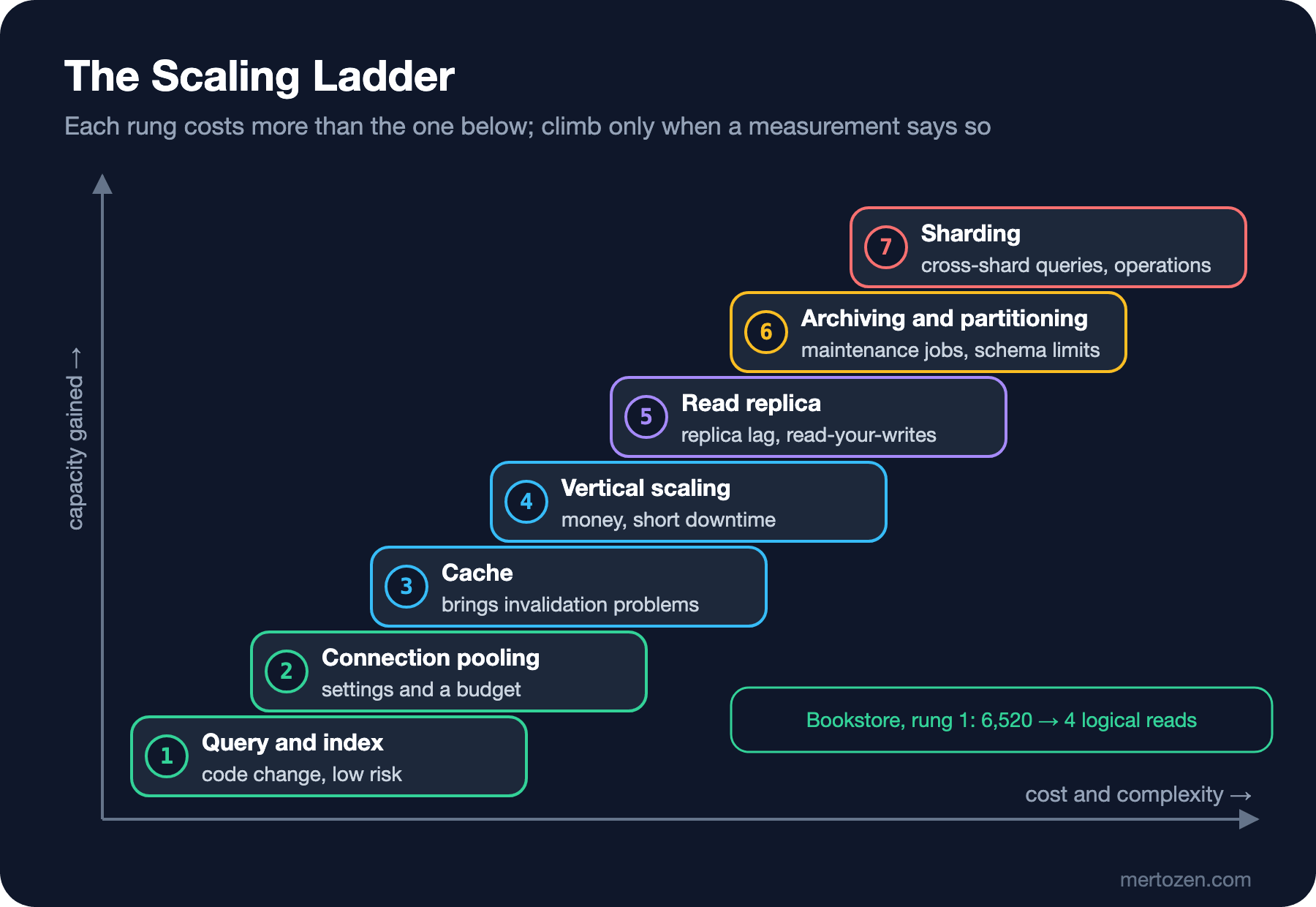
What orders the rungs is the permanent cost each one brings. The lower ones are local, reversible changes; the upper ones change the shape of the system and are hard to undo.
| Rung | What it buys | Permanent cost | In the series |
|---|---|---|---|
| Query and index | Often 10–1000 times | Write cost, index maintenance | This post |
| Connection pooling | Connection setup cost and server memory | Budget calculation, running PgBouncer | 02 |
| Cache | Takes repeated reads off the database | Invalidation, an inconsistency window | Caching series |
| Vertical scaling | More CPU, memory, IOPS | Money; it has a ceiling; short downtime when switching | 01, 05 |
| Read replica | Read capacity, reporting isolation | Replica lag, read-your-writes, routing code | 04–06 |
| Archiving and partitioning | Smaller hot data, easier maintenance | Maintenance jobs, primary key and query constraints | 03, 07, 08 |
| Sharding | Write capacity and data size | Cross-shard queries and transactions, resharding, operations | 09 |
Vertical scaling goes further today than most teams think: in the cloud you can get single instances with more than 100 vCPUs and terabytes of memory. The limit is usually cost and the dependence on a single machine rather than anything technical. A read replica scales reads but not writes; every replica re-applies all of the primary's writes. Sharding looks tempting because it's the only rung that scales writes, but sharding too early is expensive: queries that land on one shard, like "the customer's recent orders", get easier, while queries like "best sellers of the last 30 days" go to every shard, foreign keys and transactions stop at the shard boundary, and changing the schema turns into a separate deployment per shard. The system-level decisions (hash or range, consistent hashing) are in the System Design series posts "Scaling the Data Layer" and "Consistent Hashing".
Capacity Estimation: Growth, Size and SLO
To know where you stand on the ladder you need two estimates: how much the data will grow and how much the load will increase. On the data side we start with the size per row:
SELECT relname AS table_name,
       n_live_tup AS row_count,
       pg_size_pretty(pg_table_size(relid)) AS heap_size,
       pg_size_pretty(pg_indexes_size(relid)) AS index_size,
       round(pg_total_relation_size(relid)::numeric / n_live_tup) AS bytes_per_row
FROM pg_stat_user_tables
WHERE relname IN ('orders', 'order_items')
ORDER BY relname DESC;
table_name | row_count | heap_size | index_size | bytes_per_row
-------------+-----------+-----------+------------+---------------
orders | 1000000 | 130 MB | 73 MB | 213
order_items | 2493671 | 268 MB | 151 MB | 176n_live_tup is an estimate from statistics; the real count is 2,500,000. With 2.5 lines per order on average, one order including its indexes takes about 213 + 2.5 × 176 = 653 bytes. For the growth rate we look at daily orders per quarter:
SELECT date_trunc('quarter', created_at)::date AS quarter,
       count(*) AS orders,
       round(count(*) / 91.0) AS per_day
FROM orders
WHERE created_at >= timestamptz '2025-07-01'
GROUP BY 1
ORDER BY 1;
quarter | orders | per_day
------------+--------+---------
2025-07-01 | 86112 | 946
2025-10-01 | 95011 | 1044
2026-01-01 | 101823 | 1119
2026-04-01 | 108374 | 1191
2026-07-01 | 117361 | 1290
2026-10-01 | 58831 | 646The last quarter looks low because it isn't over yet. The last full quarter has 1,290 orders a day. The product team's target is 10 times in a year: about 12,900 orders a day. That is 12,900 × 365 × 653 bytes ≈ 3.1 GB of new data a year. Data size alone won't strain a server. What will is the read traffic behind every order (catalog, cart, order history, reports), the peak load on campaign days and the connections opened by many application instances. The method for rough estimates (QPS, storage, bandwidth) is in the System Design series post "Back-of-the-Envelope Estimation".
The second step is turning "the database is slow" into a measurable target. An SLO helps here: "The database query behind the My orders endpoint stays under 50 ms at p99 in 5-minute windows, including peak load on campaign days." That sentence makes it possible both to measure where we are today and to verify whether a scaling step worked. Before the index p99 was 653 ms, 13 times the target; after the index it is 5.6 ms, far below it.
The Bookstore Scenario: 10x in a Year
This is the story we follow through the series: Bookstore will grow tenfold in orders within a year, and institutional orders (bulk purchases by schools and libraries) and campaign days will make the load spiky. In each post we hit a problem and climb a rung: the connection budget as API instances multiply (02), moving four years of orders to an archive without stopping the live system (03), moving reports and read traffic to a replica (04–06), what happens to payments and orders if the primary goes down (05), partitioning the orders table (07–08) and why sharding isn't needed at this stage (09–10). At every step we measure first, then decide, then verify with the same metric.
Production Notes
Make measurement continuous. The production counterpart of this post's sampler and pg_stat_statements query is metrics shipped to a monitoring system every minute: calls and duration per query, the wait distribution of active sessions, connection count, replica lag. When something goes wrong, having the answer to "what was it" in historical data saves hours.
Measure on the application side too. The time the database sees is only part of the time the user sees; waiting for a connection from the pool, the network and reading the result set don't show up in database metrics. In .NET, OpenTelemetry traces that go from the endpoint down to the query show the difference.
Aggregate percentiles correctly. The average of several instances' p99 values is not a p99. Use a metrics system that keeps histograms or combine the raw durations.
Be careful when carrying lab results into production. The numbers here were taken on a single machine with the data mostly in memory. In production disk, network and other workloads come into play; repeat the same method in your own environment with real data sizes.
Common Pitfalls
Looking at average latency: the average hides the long tail that produces the most complaints. Watch at least p95 and p99.
Reading throughput without the client count: "187 requests per second" says nothing on its own. If the same throughput takes 32 ms with 4 clients and 327 ms with 64 clients, the second one is a saturated system.
Covering a query problem with hardware: moving a query that scans a table to a machine with twice the CPU brings twice the gain at best; the index brought 130 times. Before deciding on vertical scaling or a replica, look at the plans of the most expensive queries.
Sharding too early: building a sharded system for 3 GB of yearly growth is a permanent cost that slows down all later development. The sharding decision comes from measurements of write capacity and data size, not from growth expectations.
Building test data with the wrong distribution: test data where everyone has a single order or every date falls on the same day doesn't show how indexes and plans behave in reality. The data in this post is spread over four years and concentrated in the recent quarters.
A Small Experiment
★☆☆ Drop the index and run the load with 8 clients, then turn off parallel scans with ALTER DATABASE bookstore SET max_parallel_workers_per_gather = 0 and repeat. Compare the effect of the parallel scan on throughput and p99.
★★☆ Add a second scenario to the load command: a single order detail by order_id. Plot the throughput curves of both scenarios at the same concurrency levels and compare where they bend.
★★★ Run the sampler against SQL Server as well and measure how the share of CXCONSUMER changes with the client count without the index. Then repeat with ALTER DATABASE SCOPED CONFIGURATION SET MAXDOP = 1 and explain the result with Little's Law.
In the next post we climb the second rung: connection pooling. We'll measure how the ADO.NET pool works, the real causes of the "max pool size reached" error, how multiplying API instances can overwhelm a database, and the traps that come with putting PgBouncer in front of PostgreSQL.