

Choosing a Vector Database: pgvector, SQL Server 2025, Qdrant, Azure AI Search and Elasticsearch
Try your existing database's vector support first, and tune the ANN index by measuring recall on your own data. On a 100,000-vector pgvector table exact search took 237 ms and HNSW 1 ms, but recall stayed at 0.83 with the default ef_search; with a filter, HNSW forced onto the index returned zero rows while an iterative scan found 10. HNSW, IVFFlat, DiskANN, choosing a metric, and five options compared.
Version note: The code in this post was built and run with .NET 10, Npgsql 10.0.3 and Pgvector 0.3.2 against PostgreSQL 17.11 and pgvector 0.8.7 (Docker image pgvector/pgvector:pg17).
Guess First
A table holds 100,000 vectors of 768 dimensions with an HNSW (Hierarchical Navigable Small World) index on top. Every row has a category column; category = 7 selects about 2% of the rows. You run this query: "among rows in category 7, return the 10 vectors closest to the query". If the index is used, how many rows come back? 10, or fewer?
The answer opens one of the most important questions to ask when choosing a vector database: how do you combine a filter with ANN (Approximate Nearest Neighbor) search?
Exact kNN and ANN
The search we did over the in-memory list was exact kNN (k-Nearest Neighbors): compare the query vector with every vector and take the k closest. The result is exact and the cost grows linearly with the row count. In the second post we saw that brute-force scanning 100,000 vectors in C# takes 14 ms at 768 dimensions; in a database the same work costs more, disk reads included. For this table an exact search in PostgreSQL took 237 ms per query on average.
ANN indexes give up a little exactness to gain speed: they find most of the 10 closest vectors without looking at every vector. You measure how many they find with recall: how many of the 10 vectors in the exact result also appear in the ANN result. A recall of 0.95 means one of every 20 true neighbors is missed. For RAG (Retrieval-Augmented Generation) that means "sometimes the right chunk never arrives", so you should not pick index parameters without measuring recall.
Index Types: HNSW, IVFFlat, DiskANN
HNSW places vectors in a layered graph. The bottom layer contains every vector, each linked to its nearest neighbors; upper layers have fewer and fewer nodes with long-range links. A search starts from the entry point at the top, jumps on each layer to the neighbor closer to the query, drops a layer, and at the bottom collects the closest ones while keeping a candidate list.
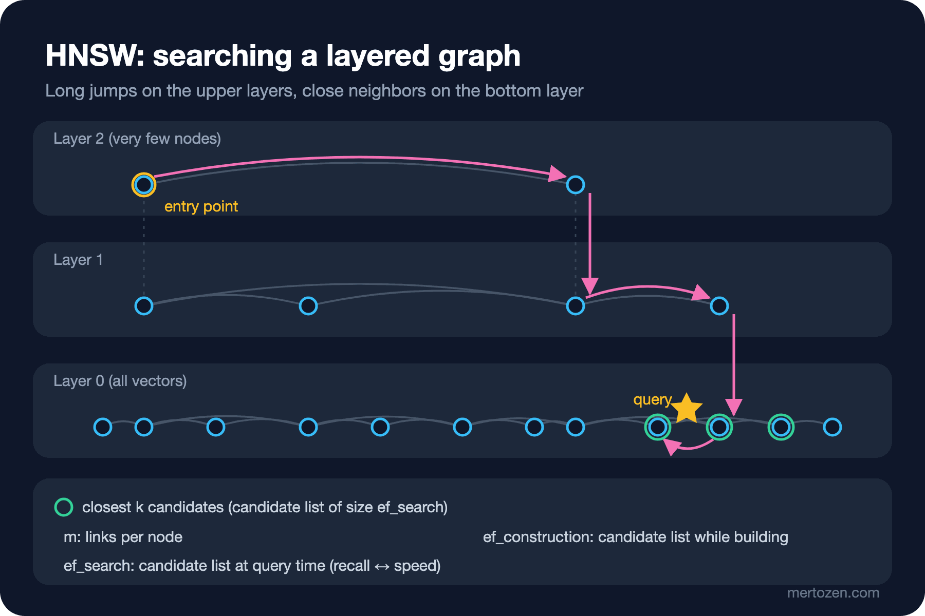
Three parameters drive this behavior. m sets how many links each node has, ef_construction how many candidates are considered while building the index; both make the index bigger and the build slower but raise recall. ef_search is the size of the candidate list at query time and can be changed per session without rebuilding the index. pgvector's defaults are m = 16, ef_construction = 64 and hnsw.ef_search = 40.
IVFFlat (Inverted File with Flat compression) splits vectors into lists clusters with k-means; at query time it only looks inside the probes clusters closest to the query. It builds faster, but because the clusters are learned from the data when the index is built, you should not build it on an empty table. The pgvector README suggests starting with lists = rows / 1000 for up to a million rows and the square root of lists for probes; the default probes is 1.
DiskANN is a graph-based ANN method from Microsoft Research, designed to keep most of the graph on SSD (Solid-State Drive). SQL (Structured Query Language) Server 2025's vector index uses it; we cover it in the sixth post.
Measuring with 100,000 Vectors
I used synthetic data instead of real embeddings, because embedding 100,000 chunks with a local model would take hours. 200 random cluster centroids and 500 points scattered around each with noise:
/* 200 cluster centroids, 768 dimensions each */
CREATE TABLE bench_centroids AS
SELECT c, ARRAY(SELECT (random() - 0.5)::real FROM generate_series(1, 768) WHERE c > -1) AS v
FROM generate_series(0, 199) c;

/* 100,000 points: centroid + noise; category is a random filter column with 2% per value */
CREATE TABLE bench_items (id int PRIMARY KEY, category int NOT NULL, embedding vector(768) NOT NULL);
INSERT INTO bench_items
SELECT i, floor(random() * 50)::int,
       (SELECT array_agg(x.val + (random() - 0.5) * 0.6 ORDER BY x.ord)
        FROM unnest(c.v) WITH ORDINALITY AS x(val, ord))::vector
FROM generate_series(1, 100000) i
JOIN bench_centroids c ON c.c = i % 200;
This SQL produced a 403 MB table in 12 seconds. The measurement program creates 50 query vectors that are not in the table (centroid plus fresh noise), first gets the exact results without an index, then builds the index and runs the same queries with different parameters:
// Exact kNN: without an index the result is exact and is the recall reference
(List<HashSet<int>> truth, double exactMs) = await SearchAllAsync(conn, queries, null);
Console.WriteLine($"exact (seq scan)          recall@10=1.000  avg={exactMs:F1} ms");

Stopwatch sw = Stopwatch.StartNew();
await Exec(conn, "SET maintenance_work_mem = '1GB'; CREATE INDEX bench_hnsw ON bench_items USING hnsw (embedding vector_cosine_ops) WITH (m = 16, ef_construction = 64);");
Console.WriteLine($"hnsw build: {sw.Elapsed.TotalSeconds:F1} s, size: {await Scalar(conn, "SELECT pg_size_pretty(pg_relation_size('bench_hnsw'))")}");

foreach (int ef in new[] { 10, 40, 100, 200 })
{
    await Exec(conn, $"SET hnsw.ef_search = {ef}");
    (List<HashSet<int>> got, double ms) = await SearchAllAsync(conn, queries, null);
    Console.WriteLine($"hnsw ef_search={ef,-4}       recall@10={Recall(truth, got):F3}  avg={ms:F1} ms");
}

private static async Task<(List<HashSet<int>>, double)> SearchAllAsync(NpgsqlConnection conn, List<Vector> queries, int? category)
{
    string where = category is null ? "" : "WHERE category = @cat";
    List<HashSet<int>> results = [];
    Stopwatch sw = Stopwatch.StartNew();
    foreach (Vector q in queries)
    {
        await using NpgsqlCommand cmd = new($"SELECT id FROM bench_items {where} ORDER BY embedding <=> @q LIMIT 10", conn);
        cmd.Parameters.AddWithValue("q", q);
        if (category is not null) cmd.Parameters.AddWithValue("cat", category.Value);
        HashSet<int> ids = [];
        await using NpgsqlDataReader r = await cmd.ExecuteReaderAsync();
        while (await r.ReadAsync()) ids.Add(r.GetInt32(0));
        results.Add(ids);
    }
    return (results, sw.Elapsed.TotalMilliseconds / queries.Count);
}

private static double Recall(List<HashSet<int>> truth, List<HashSet<int>> got) =>
    truth.Zip(got, (t, g) => (double)t.Intersect(g).Count() / t.Count).Average();
<=> is pgvector's cosine distance operator. The results:
$ dotnet run -c Release -- vdb-bench
exact (seq scan)          recall@10=1.000  avg=237.6 ms
hnsw build: 31.3 s, size: 391 MB
hnsw ef_search=10         recall@10=0.610  avg=0.8 ms
hnsw ef_search=40         recall@10=0.830  avg=0.9 ms
hnsw ef_search=100        recall@10=0.898  avg=1.1 ms
hnsw ef_search=200        recall@10=0.898  avg=1.4 ms
hnsw + WHERE category=7   avg rows=10.0/10  avg=6.7 ms
  + iterative_scan        avg rows=10.0/10  avg=5.9 ms
ivfflat build: 10.0 s, size: 392 MB
ivfflat probes=1           recall@10=0.936  avg=1.2 ms
ivfflat probes=10          recall@10=1.000  avg=3.8 ms
ivfflat probes=32          recall@10=1.000  avg=11.6 ms
Speed first: exact search takes 237 ms, HNSW around 1 ms. More than two hundred times faster, and the gap widens as the table grows. The price is visible too: the HNSW index is 391 MB, as big as the table itself, and took 31 seconds to build. With the default ef_search = 40 recall is 0.830; roughly 2 of every 10 true neighbors are missed. Raising ef_search to 100 took recall to 0.898 and added only 0.2 ms of latency; at 200 recall did not improve.
That IVFFlat comes out better on this data should catch your eye: 0.936 with probes = 1, exactly 1.000 with probes = 10. The reason is the data: a synthetic set of 200 distinct clusters is the ideal case for a k-means based index. Real text embeddings do not cluster this neatly, so do not conclude "IVFFlat is better" from this table. The lesson is a different one: choose index parameters with your own data and by measuring recall, not with someone else's benchmark.
Choosing a Distance Metric
pgvector has three main metrics: L2 (Euclidean) distance <->, inner product <#> (returns the negative value) and cosine distance <=>. The index's operator class must match the metric: vector_l2_ops, vector_ip_ops, vector_cosine_ops. An index built with the wrong operator class is never used by the query; we will see that with EXPLAIN in the seventh post.
The embedding model tells you which one to choose. Most text embedding models are trained for cosine. If the vectors are already normalized to length 1 (Ollama's nomic-embed-text output is; we measured it in the second post), cosine, inner product and L2 produce the same ranking; the pgvector README recommends inner product in that case for best performance. With non-normalized vectors the three rank differently, and deviating from the metric the model recommends silently lowers recall.
Filters and ANN: Pre-filter, Post-filter, Iterative Scan
In RAG a filter is the rule, not the exception: tenant, permissions, document type, language, date. Back to the opening question. First, PostgreSQL's own plan:
SET hnsw.ef_search = 40;
SELECT embedding AS q FROM bench_items WHERE id = 5 \gset
EXPLAIN (ANALYZE, COSTS OFF)
SELECT id FROM bench_items WHERE category = 7
ORDER BY embedding <=> :'q' LIMIT 10;

 Limit (actual time=11.815..11.816 rows=10 loops=1)
   ->  Sort (actual time=11.814..11.815 rows=10 loops=1)
         Sort Key: ((embedding <=> '[...]'::vector))
         Sort Method: top-N heapsort  Memory: 25kB
         ->  Seq Scan on bench_items (actual time=0.007..11.674 rows=1940 loops=1)
               Filter: (category = 7)
               Rows Removed by Filter: 98060
 Planning Time: 0.049 ms
 Execution Time: 11.829 ms
(9 rows)
The planner did not use the index at all. Since the filter selects 2% of rows, it found it cheaper to scan the 1,940 rows sequentially and compute the distance only for them: 11.8 ms, and the result is exact. This is a pre-filter: filter first, then run an exact search over the filtered set. For selective filters it is often the right plan. Now let's force the planner onto the index:
SET enable_seqscan = off;
EXPLAIN (ANALYZE, COSTS OFF)
SELECT id FROM bench_items WHERE category = 7
ORDER BY embedding <=> :'q' LIMIT 10;

 Limit (actual time=3.500..3.500 rows=0 loops=1)
   ->  Index Scan using bench_hnsw on bench_items (actual time=3.499..3.499 rows=0 loops=1)
         Order By: (embedding <=> '[...]'::vector)
         Filter: (category = 7)
         Rows Removed by Filter: 40
 Planning Time: 0.085 ms
 Execution Time: 3.509 ms
(7 rows)
Zero rows. The HNSW index returned ef_search = 40 candidates, the filter removed all 40 and the query came back empty. This is a post-filter: ANN first, then the filter. The more selective the filter, the more incomplete the result. The pgvector README describes the same with its own example: for a condition matching 10% of rows, about 4 rows remain on average with the default ef_search.
pgvector 0.8.0 introduced iterative index scans for this: keep scanning the index until enough results are found.
SET hnsw.iterative_scan = relaxed_order;
EXPLAIN (ANALYZE, COSTS OFF)
SELECT id FROM bench_items WHERE category = 7
ORDER BY embedding <=> :'q' LIMIT 10;

 Limit (actual time=0.573..8.100 rows=10 loops=1)
   ->  Index Scan using bench_hnsw on bench_items (actual time=0.573..8.099 rows=10 loops=1)
         Order By: (embedding <=> '[...]'::vector)
         Filter: (category = 7)
         Rows Removed by Filter: 473
 Planning Time: 0.017 ms
 Execution Time: 8.107 ms
(7 rows)
Ten rows, 8.1 ms. The index pushed 473 candidates through the filter until it found 10 matches. relaxed_order allows small deviations in the distance order of the results; strict_order exists if you need exact ordering. To keep the scan from running forever there is a hnsw.max_scan_tuples limit (20,000 by default).
In production you need to choose deliberately among these three plans. For very selective filters (a single tenant's documents) a pre-filter with a B-tree index and exact search is usually enough and correct. When a filter has many values but each one is large, consider partial indexes or partitioning. In between, iterative scan. Always check which one is chosen with EXPLAIN; in the seventh post we try tenant and permission filters on the real doc_chunks table.
Options: pgvector, SQL Server 2025, Qdrant, Azure AI Search, Elasticsearch
If you already have a database, the first question should be "is its vector support enough for me?" A separate vector database brings new backup, monitoring, security and data synchronization problems; if the chunks' metadata and permissions live in the main database, consistency between the two systems becomes your problem too.
| Option | ANN index | Filtering | .NET access | When |
|---|---|---|---|---|
| PostgreSQL + pgvector | HNSW, IVFFlat | SQL WHERE; iterative scan since 0.8 | Npgsql + Pgvector, EF (Entity Framework) Core, Dapper | You already run PostgreSQL |
| SQL Server 2025 | DiskANN (preview) | Iterative filtering in the latest index version | EF Core 10, SqlClient 6.1 | You already run SQL Server |
| Qdrant | HNSW | Payload filters applied during search | Qdrant client | Large scale, a separate service is acceptable |
| Azure AI (Artificial Intelligence) Search | HNSW, exhaustive kNN | OData filters | Azure SDK (Software Development Kit) | You need managed hybrid search |
| Elasticsearch | HNSW | Filters inside the kNN search | Elastic client | Full-text search already lives there |
You can also reach all of them through the Microsoft.Extensions.VectorData abstraction; the provider list on Microsoft Learn has packages for PostgreSQL, SQL Server, Qdrant, Azure AI Search and Elasticsearch (CommunityToolkit.VectorData.PgVector, CommunityToolkit.VectorData.SqlServer, CommunityToolkit.VectorData.Qdrant, CommunityToolkit.VectorData.AzureAISearch, Elastic.SemanticKernel.Connectors.Elasticsearch). The API (Application Programming Interface) itself is the subject of the upcoming .NET with AI series; what matters here is that a common abstraction offers the lowest common denominator. For fine-grained settings such as pgvector's iterative scan or SQL Server's WITH APPROXIMATE, you have to go down to the database's own API or to EF Core. In this series the main example is PostgreSQL + pgvector; SQL Server 2025 gets its own post next.
Production Notes
Building an index is an operation of its own. The first time I ran this measurement, the HNSW build failed with this error:
53100: could not resize shared memory segment "/PostgreSQL.2802977584" to 1070632384 bytes: No space left on deviceA parallel HNSW build needs shared memory up to maintenance_work_mem; a Docker container's /dev/shm is 64 MB by default. The pgvector README says to set Docker's --shm-size to at least maintenance_work_mem; restarting the container with --shm-size=1g fixed it. Conversely, leaving maintenance_work_mem at its 64 MB default makes PostgreSQL emit a NOTICE, "hnsw graph no longer fits into maintenance_work_mem after 17699 tuples", and the build slows down noticeably.
Put index size into your capacity plan. For 100,000 vectors of 768 dimensions the table is 403 MB and the HNSW index 391 MB. HNSW works well only if the index fits in memory; at a million chunks these numbers grow tenfold. That is where halfvec and Matryoshka truncation from the second post turn into a concrete win.
Monitor recall. ef_search is not a number you pick once and forget; as data grows and its distribution shifts, the same value gives a different recall. Periodically comparing your measurement set against exact search lets you see a recall drop before your customers do.
Common Pitfalls
First, benchmarking with 1,000 rows. At 1,000 rows exact search is fast too, and the index gives perfect recall; the differences only show up in the hundreds of thousands and millions. Measure with data close to your target size.
Second, scanning the table without an index. Without an index every query scans the whole table; 237 ms at 100,000 rows, seconds at a million. Verify with EXPLAIN that the index is used.
Third, combining a filter with ANN and not checking the result count. An empty or incomplete result from a post-filter raises no error; the RAG context simply stays empty and the model says "I don't know".
Fourth, generalizing from a synthetic benchmark. The IVFFlat result in this post is a consequence of the data's cluster structure; real embeddings may not rank the same way.
Fifth, adding a separate vector database just because "we need a vector database". Synchronizing document deletes, permission changes and re-embedding between two systems takes more work than the search itself.
A Small Experiment
★☆☆ Create a B-tree index on category in bench_items and look at the plan of the opening query again. Which plan does the planner choose, and how much does the time change?
★★☆ Rebuild the HNSW index with m = 32, ef_construction = 128. How do build time, index size and recall at ef_search = 40 change?
★★★ Regenerate bench_items with 2,000 clusters instead of 200 (50 points per cluster). Does the recall ranking of IVFFlat and HNSW change? Interpret the result in terms of how the structure of the data affects index choice.
We have seen the options and the mechanics of ANN. In the next post we move to SQL Server 2025's vector type and EF Core's VectorDistance support; then in the seventh post we do the same work with PostgreSQL and pgvector on our real document chunks.