

Interpreting Results: Percentiles, Coordinated Omission, the Throughput-Latency Curve and Finding the Bottleneck
Reading a load test correctly means looking at percentiles instead of the average, never averaging percentiles, using the open model to avoid coordinated omission, looking for capacity at the knee of the throughput-latency curve and finding the bottleneck with the USE method. We freeze the Bookstore API for 5 seconds and measure a closed-model p99 of 8 ms against an open-model 4.2 seconds, then trace the curve's collapse to the connection pool and SQL Server waits.
Version note: The code in this post was built and run with .NET 10; the load tests were run with k6 2.4.0 against Bookstore.Api and SQL Server 2025 on Docker Compose, and runtime measurements were taken with dotnet-counters 10.0.750501.
Guess First
The API of Bookstore, the online bookstore used as the shared example across this site's series, freezes for 5 seconds on a campaign evening; it could be a GC pause, a VM migration or a log file being flushed to disk. Two teams measure the same minute. In one test 20 virtual users wait for a response and then send a new request (closed model); in the other, 200 requests per second arrive at a fixed rate (open model). Do you think the two tests report a similar p99? Second question: if you average the p99 values k6 gives for every 10 seconds, do you get the p99 of the minute? Third: can the system drop to 125 requests per second with a 34-second p95 while the API's CPU hovers around 30 percent? In this post we talk about reading numbers correctly, with real measurements.
Why the Average Misleads
The open-model result of the freeze experiment above is this: average 180.5 ms, median (p50) 0.47 ms, p95 1.54 seconds, slowest request 5.13 seconds. The average describes no request at all. Most requests come back in half a millisecond, about 700 take seconds. The average falls between the two groups, at a place nobody experienced. Response-time distributions are almost never symmetric: they have a long right tail, and the tail is what bothers users.
A percentile is a way to read the distribution at one point: p95 = 1.54 seconds means 95 percent of requests completed in that time or less. p50 describes the typical request, p95 and p99 the tail, and max a single request. Do not rely on max alone; it is the number that moves most from run to run. The number of requests per page raises the importance of the tail. If a page makes 20 API calls in a system where each call is slow with a probability of 1 percent, about 18 percent of pages contain at least one slow call (1 minus 0.99 to the 20th power, about 0.18). So p99 is not "one user in a hundred has a problem".
Percentiles Cannot Be Averaged
I computed p99 separately for every 10 seconds of the same run:
open p99 per 10s: [1.3, 1.1, 1.6, 5057.6, 2.3, 2926.6, 1.2] avg= 1141.7 overall= 4230.6The average of the windows' p99 values is 1,141.7 ms; the real p99 of all requests is 4,230.6 ms. The difference is no accident. A percentile is based on ordering, and the p99 of a combined distribution cannot be computed from the p99 values of two distributions. Turning per-minute p99 values into an hourly average on a dashboard, or averaging the p95 values of the two runner pods in post 04, is the same mistake. The right way is to keep the distribution itself and merge it. A histogram does that: it counts values into buckets, and the buckets of two histograms can be added. HdrHistogram, Gil Tene's histogram library that keeps a wide value range at a fixed precision, is a widely used structure for this. The histograms sent by k6's OpenTelemetry output (post 04) can be merged for the same reason.
Measuring Coordinated Omission
The term coordinated omission comes from Gil Tene. In short: a closed load generator holds back new requests when the system slows down. The requests that would have experienced the slow moment are never sent and drop out of the measurement. We saw this in throughput in post 01; here I measure its effect on percentiles. The scenario:
import http from 'k6/http';
import { check, sleep } from 'k6';

// Coordinated omission experiment: the same ~200 requests/s as a closed and as an open model,
// while the API is paused for a few seconds in the middle of the test (docker pause).
// Usage: k6 run -e MODEL=closed pause.js   |   k6 run -e MODEL=open pause.js
const BASE_URL = __ENV.BASE_URL || 'http://localhost:5080';
const MODEL = __ENV.MODEL || 'open';
const isbns = ['9780441172719', '9780261102217', '9780141439587', '9780451524935', '9780060850524'];

const scenarios = {
    // 20 users, each waits 100 ms after a response: ~200 requests/s while the API is fast.
    closed: { executor: 'constant-vus', vus: 20, duration: '60s' },
    open: { executor: 'constant-arrival-rate', rate: 200, timeUnit: '1s', duration: '60s', preAllocatedVUs: 50, maxVUs: 2000 },
};

export const options = { scenarios: { [MODEL]: scenarios[MODEL] } };

export default function () {
    const isbn = isbns[Math.floor(Math.random() * isbns.length)];
    const res = http.get(`${BASE_URL}/api/books/${isbn}`, { tags: { name: 'GET /api/books/{isbn}' } });
    check(res, { 'book 200': (r) => r.status === 200 });
    if (MODEL === 'closed') {
        sleep(0.1);
    }
}
k6 run -e MODEL=closed pause.js
# 30 s after the test starts, in a second terminal:
docker pause $(docker compose ps -q api); Start-Sleep 5; docker unpause $(docker compose ps -q api)== closed
http_req_duration..............: avg=10.76ms min=194µs med=1.14ms max=4.98s p(90)=2ms p(95)=2.65ms p(99)=8.1ms
http_reqs......................: 10717 178.428909/s
== open
http_req_duration..............: avg=180.54ms min=165µs med=468µs max=5.13s p(90)=1.69ms p(95)=1.54s p(99)=4.23s
http_reqs......................: 11510 191.82379/s
dropped_iterations.............: 491 8.182926/s| Measurement | Requests | Slower than 1 s | p95 | p99 |
|---|---|---|---|---|
| Closed model | 10,717 | 20 | 2.65 ms | 8.1 ms |
| Closed model, corrected | 11,597 | - | 1,763.6 ms | 4,428.4 ms |
| Open model | 11,510 | 702 | 1.54 s | 4.23 s |
The answer to the first guess question: both tests went through the same 5-second freeze, but the closed test's p99 is 8 ms and the open test's is 4.2 seconds. In the closed test, 20 requests from 20 users waited during the freeze; no new requests came because the other users were already waiting for responses. Only 20 of 10,717 requests are slow, two in a thousand; they do not even reach p99. In the open test, 200 requests kept arriving every second during the freeze; 702 requests took longer than 1 second. Real users behave like the second test.
The closed test's result can be corrected. HdrHistogram's approach is this: each virtual user normally sent a request every 112 ms (response time plus a 100 ms wait). A request that took 4,980 ms also tells you that requests which should have been sent during that time were not: synthetic values decreasing in 112 ms steps, 4,868 ms, 4,756 ms and so on, are added. I applied this correction to k6's CSV output with a small Python script. The corrected p99 came out at 4,428 ms, very close to the open test's 4,230 ms. k6 does not apply this correction. The real fix is not correcting but using the open model from the start; the correction only helps estimate what you missed when all you have is the result of a closed test.
Ways to notice coordinated omission: check whether throughput drops in the closed test (the difference between 178/s and 191/s here is the missing requests), look at the gap between max and p99 (a 5-second max next to an 8 ms p99 is suspicious), and compare server-side metrics with the client side. The reverse happens too: the server's own histogram measures a request after it enters the application; time spent waiting in a queue does not appear there. In the "Diagnose, Fix, Prove" case of the Profiling series, the server's p99 was 6 ms while k6's was 537 ms.
The Throughput-Latency Curve and the Knee
The way to find the capacity limit is to raise the arrival rate step by step and record the achieved throughput and timings at each step. This is the measured version of the breakpoint test from post 01:
const stages = [];
for (let i = 0; i < STEPS; i++) {
    const rate = START + i * STEP;
    stages.push({ target: rate, duration: '1s' });          // jump to the next rate
    stages.push({ target: rate, duration: STEP_DURATION }); // hold it
}

export const options = {
    scenarios: {
        steps: {
            executor: 'ramping-arrival-rate',
            startRate: START,
            timeUnit: '1s',
            preAllocatedVUs: 50,
            maxVUs: 2000,
            stages,
        },
    },
};

export default function () {
    // A unique query string bypasses the output cache: every request reaches the API and the database.
    const isbn = isbns[Math.floor(Math.random() * isbns.length)];
    const res = http.get(`${BASE_URL}/api/books/${isbn}?run=${__VU}-${__ITER}`, { tags: { name: 'GET /api/books/{isbn}' } });
    check(res, { 'book 200': (r) => r.status === 200 });
}
k6 run -e START=100 -e STEP=100 -e STEPS=10 -e STEP_DURATION=20s --out csv=steps.csv steps.jsThe API is limited to 0.5 CPU; I bypassed the output cache on purpose by adding a different query string to every request, because what I want to measure here is the origin's capacity. I dropped the first 6 seconds of every step and computed the rest from k6's CSV output:
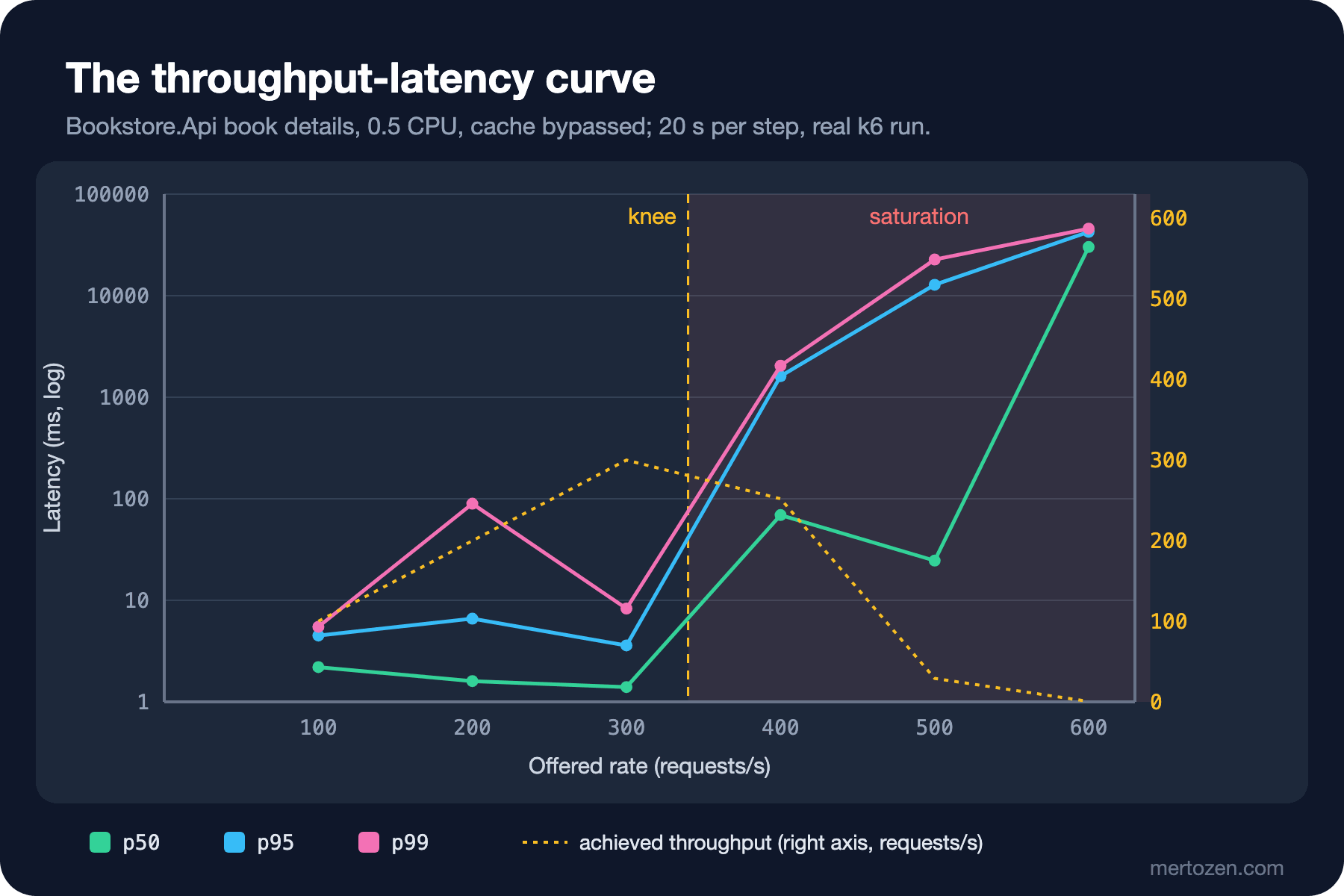
The curve has two regions. Up to 300 requests per second the achieved throughput follows the arrival rate and timings are flat: p50 1.4-2.2 ms, p95 4-7 ms. The 89 ms p99 at 200 is the effect of a few slow requests in a single step. At 400 the picture changes: the system completes only 252 requests per second, 1,094 iterations cannot start and p95 jumps to 1.6 seconds. This point between 300 and 400 is called the knee. Beyond the knee the arrival rate exceeds capacity, so the queue grows without bound; by Little's Law, timings keep rising with the amount of waiting work. In this run something worse happened: at 500 and 600 throughput fell almost to zero instead of rising. The system did not just slow down, it collapsed. We find the reason in the next section.
The capacity-planning reading is this: in production, run below the knee and leave the gap for sudden load. In this system 300 requests per second is fine and 400 is not; keeping the target load around 200-250 and tuning autoscaling to that level is reasonable. The capacity math itself is in the System Design series post "Back-of-the-Envelope Estimation".
Finding the Bottleneck with the USE Method
The USE method, Brendan Gregg's way of scanning system resources one by one, asks three questions per resource: how busy is it (utilization), is work waiting (saturation), are there errors. For Bookstore the resource list is: the API container's CPU, the .NET thread pool, the SqlClient connection pool and SQL Server. I applied 400 requests per second again for 40 seconds and measured these resources at the same time. The output below is my summary of the k6 summary, the cgroup counters, the dotnet-counters CSV and SQL Server's wait statistics (the difference of sys.dm_os_wait_stats before and after the test). I started the API container with a Docker target that includes dotnet-counters (the diag stage in the Dockerfile):
$env:API_TARGET = "diag"; $env:API_CPUS = "0.5"
docker compose up -d --build api

docker compose exec api /tools/dotnet-counters collect -p 1 --refresh-interval 5 --format csv -o /tmp/c.csv `
    --duration 00:00:35 --counters System.Runtime,Microsoft.AspNetCore.Hosting,Microsoft.Data.SqlClient.EventSource
docker compose exec api cat /sys/fs/cgroup/cpu.stat
k6: target=400 rps=125 p50=1750.76 p95=34375.32 dropped=11279 vus=2000
cpu.stat: cpu=0.14 throttled=19%
time cpu active.req pool.in.use
14:11:24 0.20 1638 78
14:11:29 0.10 2000 81
14:11:34 0.08 2000 83
14:11:39 0.01 2000 86
14:11:44 0.02 2000 88
wait THREADPOOL 1420267 ms 7604 waits
wait RESOURCE_SEMAPHORE_QUERY_COMPILE 1961056 ms 776 waits
wait CMEMTHREAD 454818 ms 599 waits| Resource | Utilization | Saturation | Errors |
|---|---|---|---|
| API CPU (0.5 limit) | 0.14 CPU on average, dropping to 0.01 over time | throttled in 19 percent of periods | none |
| .NET thread pool | low | queue practically empty | none |
| HTTP requests | - | 2,000 active requests (k6's ceiling) | timeouts |
| SqlClient connection pool | 78-88 of the 100-connection pool in use | requests waiting for a connection | "Timeout expired ... obtaining a connection from the pool" |
| SQL Server | container CPU high | THREADPOOL and RESOURCE_SEMAPHORE_QUERY_COMPILE waits | - |
The answer to the third guess question is in the table. The API's CPU is idle; the bottleneck is not in the API. While requests wait for the database they hold connections from the connection pool, the pool fills up, new requests queue for a connection and fail when SqlClient's 15-second wait expires. Over the tests in this section that error appeared 33 thousand times in the API log. The THREADPOOL wait on the SQL Server side shows that SQL Server could not find worker threads to run incoming work; so the resource is SQL Server itself. On this machine the SQL Server container shared the CPU with other workloads, and the machine's load average was around 10 during the tests. That is the mechanism behind the collapse at the 500-600 steps: when the database slows down the pool runs dry, when the pool runs dry requests time out and throughput falls to zero. How to read wait statistics is in the SQL Server Deep Dive series post "A Diagnostic Method", and finding the hot path inside the code is the topic of the "Profiling and Diagnostics in .NET" series.
The value of USE is in its order: first you quickly answer the three questions for every resource, then you look deeply only at the suspicious one. In this example, had I started by profiling the API, I would have been looking for a hot path in a process that was sitting idle.
Comparing Runs
When I repeated the same stepped test at different times, the 200 requests per second step gave a p95 of 6.6 ms in one run and 17 seconds in another. Code and configuration were the same; what changed was the other workload on the machine. The slow closed-model test in post 01 also came out at a p95 of 1.49 s and 944 ms in two runs. This is not an exception, it is the nature of measurement. Follow these rules when comparing: repeat every run at least three times and report the range, not the number of a single run. Reset the environment between runs (cache, database, containers). Make sure the two runs you compare were made in the same environment, with the same data, close in time. Keep the environment note together with the result. A report template helps too:
- Goal: which question you are answering and the acceptance criteria (thresholds derived from the SLO).
- Load: workload model, rate, duration, open or closed model, test data.
- Environment: commit, build, resource limits, data size, where the load generator ran, other work running at the same time.
- Result: p50/p95/p99 per endpoint, error rate, dropped iterations; how many repetitions and the range.
- Bottleneck: the result of the USE scan and its evidence.
- Action: what will change and how it will be verified in the next run.
Production Notes
The same rules apply to production dashboards: show percentiles instead of averages, do not average percentiles over time; compute them from histogram metrics. Remember that a server-side duration metric does not see time spent waiting in a queue; read it together with client-side measurement (synthetic tests, real user monitoring). Set alert thresholds by the knee: acting when saturation signals appear (the thread pool queue, waiters in the connection pool, dropped_iterations) gives better results than acting when utilization crosses 70 percent.
Common Pitfalls
- Reporting the average time and missing the tail.
- Averaging per-minute p99 values, or averaging the runners' p95 values.
- Ignoring the gap between max and p99 in a closed-model test.
- Saying "timings are fine" while throughput drops: in a collapsing system the few requests that complete can be fast.
- Starting the bottleneck hunt with the process whose CPU looks high; look at every resource in turn with USE.
- Reporting the number of a single run as a firm result; write down the repetition count and the range.
A Small Experiment
★☆☆ Run pause.js in the closed model with 200 VUs instead of 20 and a 1-second think time. How did the number of slow requests and p99 change during the freeze?
★★☆ Run steps.js with the output cache in play (remove the query string) and the same steps. Where did the knee move? Measure the cache's hit ratio with the method from post 02.
★★★ Shrink the API's connection pool with Max Pool Size=20 and repeat the stepped test. How did the knee and the collapse point change? Fill in the USE table again and discuss the right pool size.
A load test shows how the system behaves as a whole. Sometimes the problem is a single method getting a few hundred nanoseconds slower, and that cannot be seen in the noise of a load test. In the last post of the series we move to advanced BenchmarkDotNet: parameters, baselines, diagnosers, comparing .NET 10 with .NET 11 and catching regressions in CI.